Actual fire rate of an amoeba
First of all we should note that although the fire rate of each amoeba is
 , the actual rate is different because of the fact that after firing a wave
the amoebae fall to a refractory state for M time steps.
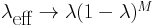
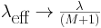
The effective fire rate will be denoted by
, the actual rate is different because of the fact that after firing a wave
the amoebae fall to a refractory state for M time steps.
The effective fire rate will be denoted by
 and it can be shown to be
 This value aggrees with the intuitive observations that as
 then
then
 and as
 then
then
 The following figures show the relation between
and
for different values
of M.
The following figures show the relation between
and
for different values
of M.
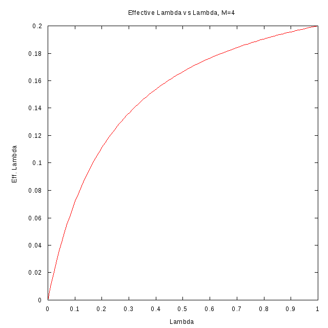
M=4
|
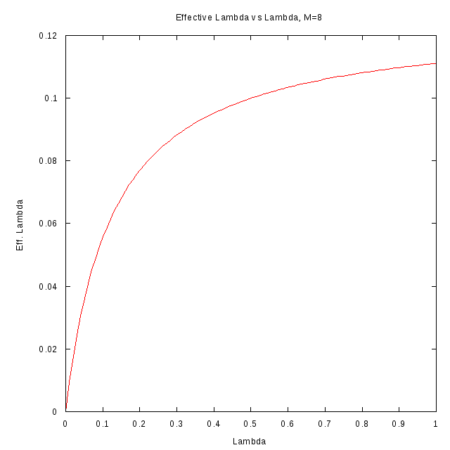
M=8
|
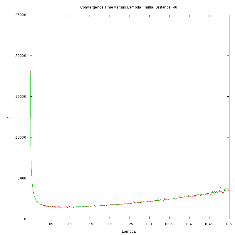
Optimal fire rate for the case of two amoebae
In this section we present some results on the study of the aggregation
time of two amoebae.
The first set of results are for M=4.
The procedure we followed in order to obtain the results was the following:
- For each initial distance D, we measured the average time required for the amoebae to converge,
by using 150 experiments, for different values of the fire rate
- After fiting the data we performed a numerical differentiation on the fited polynomial
in order to identify the value of

The results we obtained are displayed in the following table
D=40 cells
|
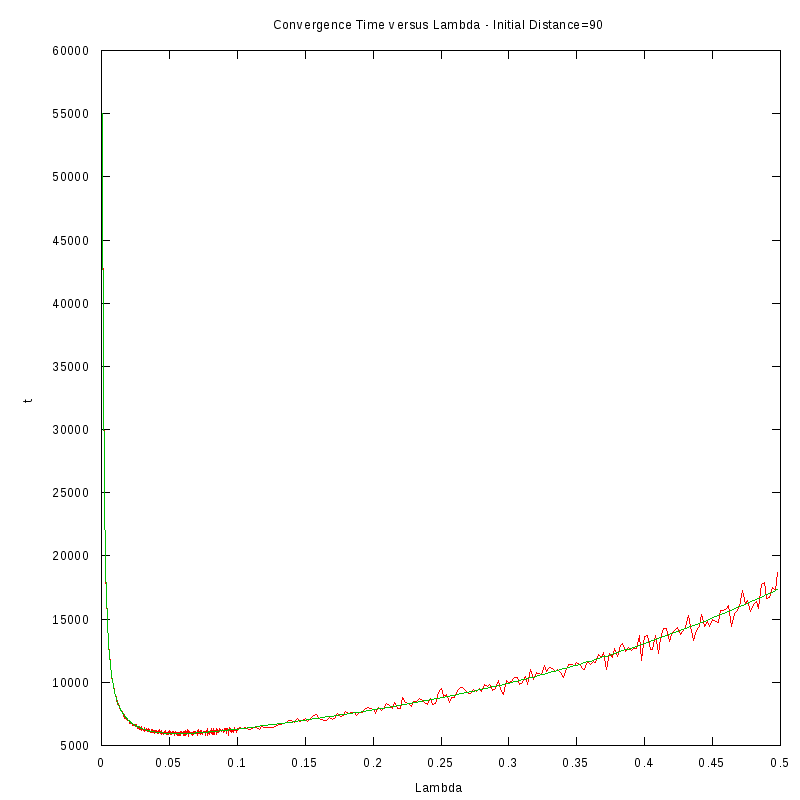
D=90 cells
|
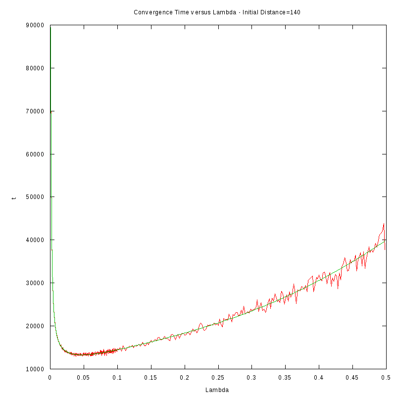
D=140 cells
|
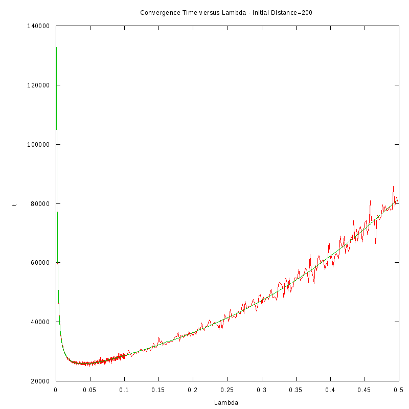
D=200 cells
|
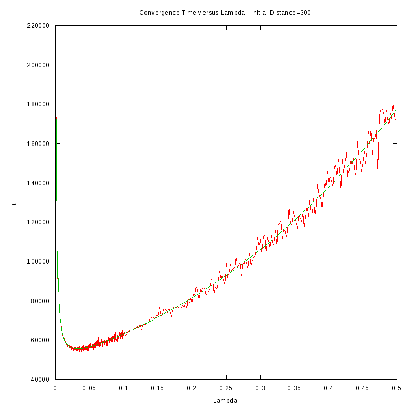
D=300 cells
|
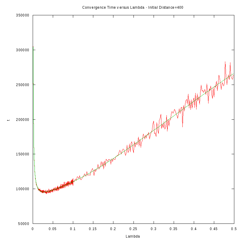
D=400 cells
|
The relationship between D and
is shown in the following picture:
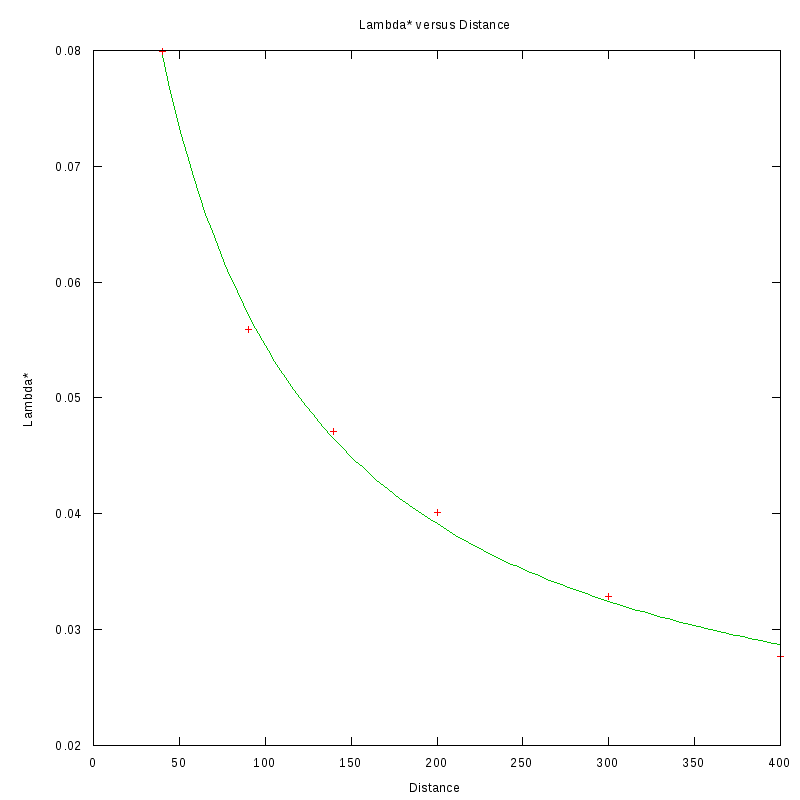 As we can see, the value of Lambda star is in very good agreement with an inverse proportionality law
with respect to the distance (the actual fitted curve is of the form
As we can see, the value of Lambda star is in very good agreement with an inverse proportionality law
with respect to the distance (the actual fitted curve is of the form
 ).
A possible hypothesis that explains this behavior is the following:
).
A possible hypothesis that explains this behavior is the following:
In the optimal case, there should be only a single wave present in the area that is between the two amoebae.
Using
, the average waves emitted in a time interval Δτ are
*Δτ. Taking Δτ = D and following what we mentioned above that there should be
only 1 wave present we can conclude that λeff*D ≈ 1.
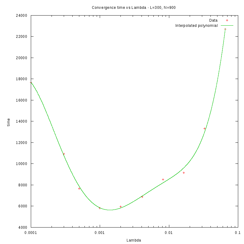
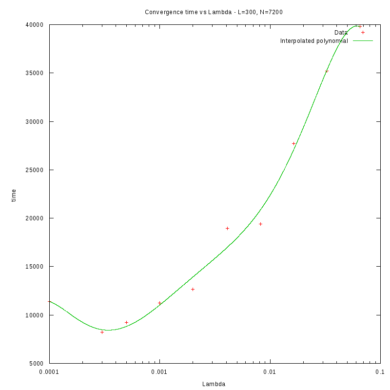
Convergence Time versus Distance in the two amoebae case
The following experiments study the time required for two amoebae to converge
given their initial distance.
The amoebae are not studied close to the λ* region, since we
are interested in seeing how the time scales for the two cases,
<<
and
>>
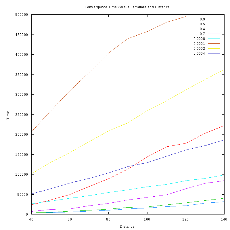
Convergence time for different
λ and distances
|
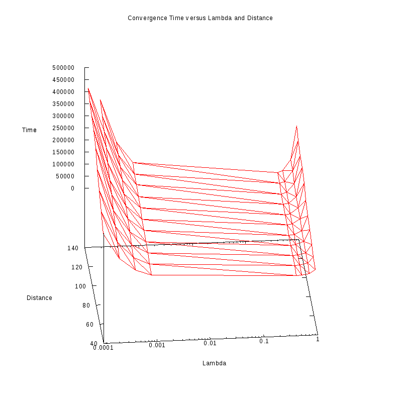
Same plot in 3D with
log-scale λ axis
|
Our main observation regarding these results is that from a first view, the convergence time seems to scale linearly with
distance for small values of
while for values much greater than
some non-linearities emerge
(note that most probably the reason for the non-linearities in the curve for
=0.0001 is the fact that the values for the
time of convergence were close to the maximum time we allowed our experiments to run, which leads to some kind of "saturation"
of the curve).
Of course, further experiments need to be performed to verify these non-linearities and ensure that the small
curves do not
appear linear simply because we observe them in a small scale.
Average time that a wave requires to reach an amoeba (2-amoebae case)
The following experiments aimed at measuring the average time that was required for a wave
to reach either one of the two amoebae.
In all experiments, M=4.
The experiments were run on an FPGA (TODO: link to sources???)
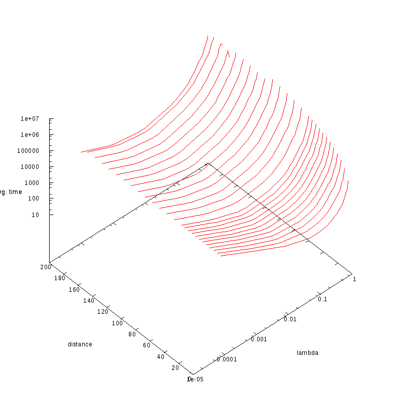
Average wave time vs
and distance (double logarithmic scale)
|
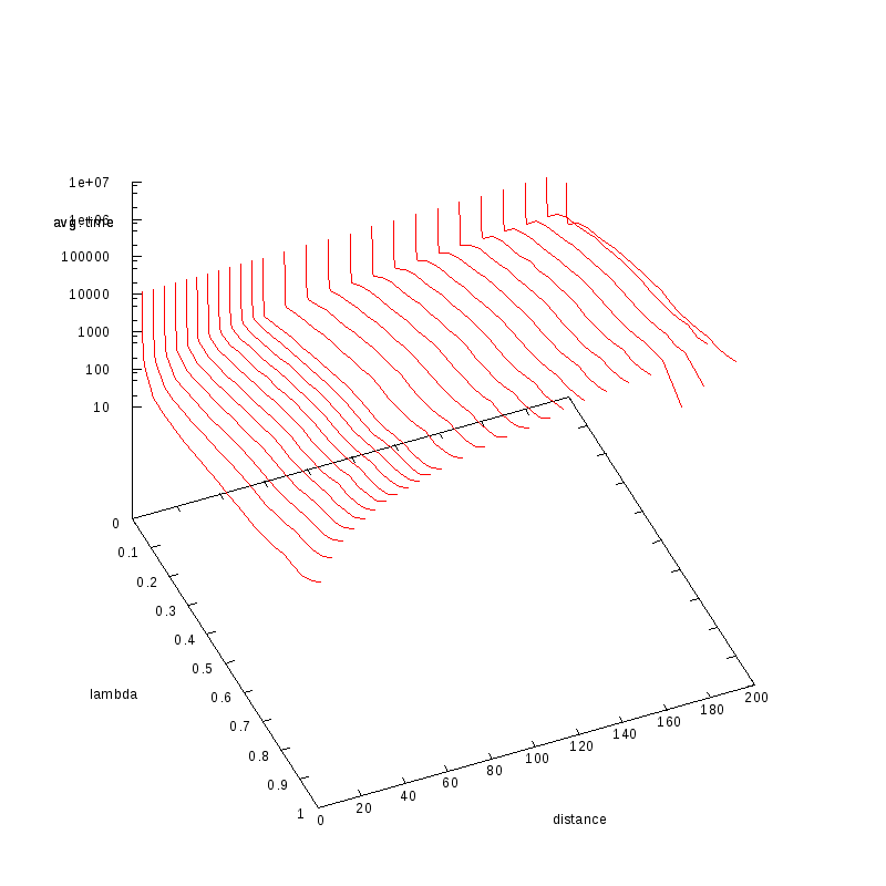
Same plot with only logscale in Z (time)
|
Position versus Time
Experiments with two clusters
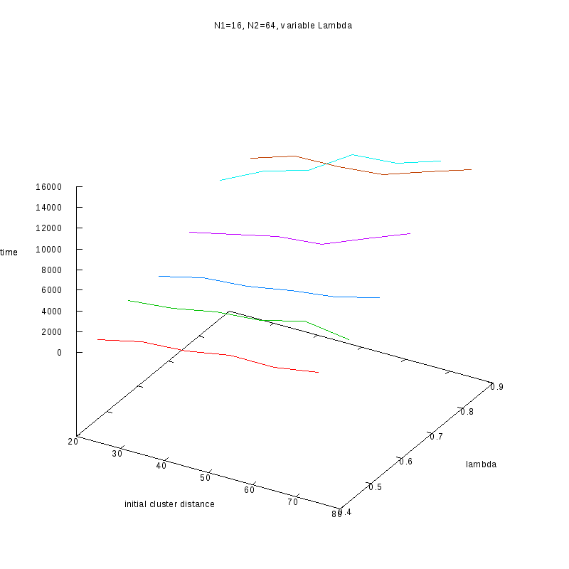
In this section we will discuss some of the results that we obtained while
experimenting on the scaling behavior of two clusters of the same or different
sizes, and attempt to make some comparisons with the case of the two single
amoebae.
Note that, although we performed approximately 250 iterations per experiment,
the resulting curves exhibit increased noise.
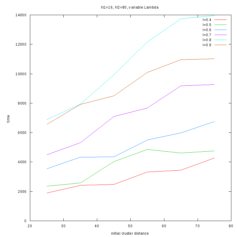
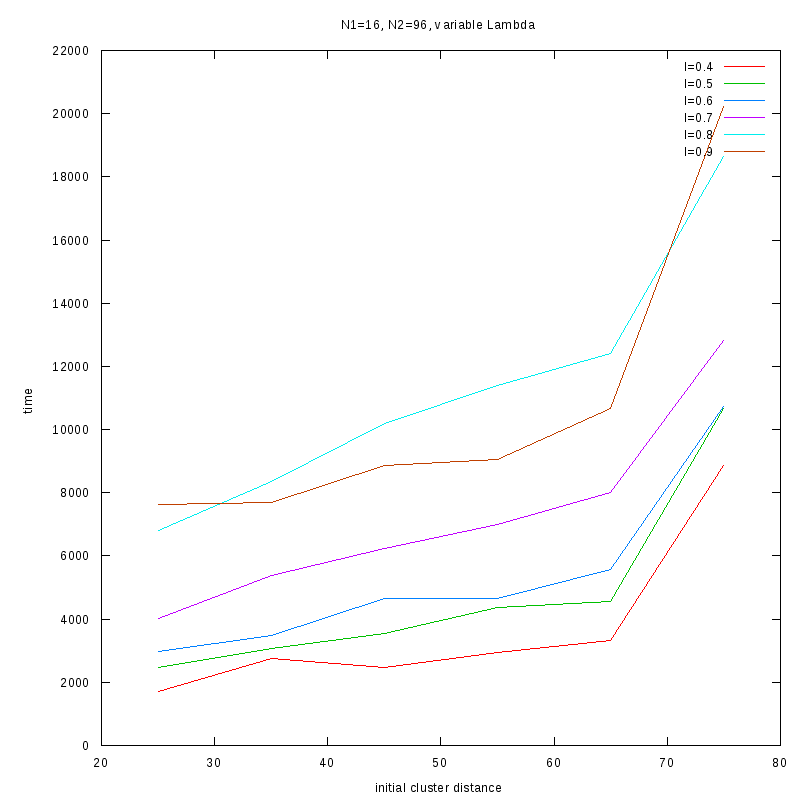
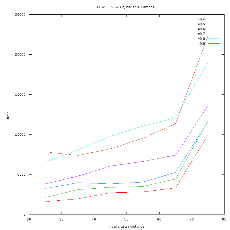
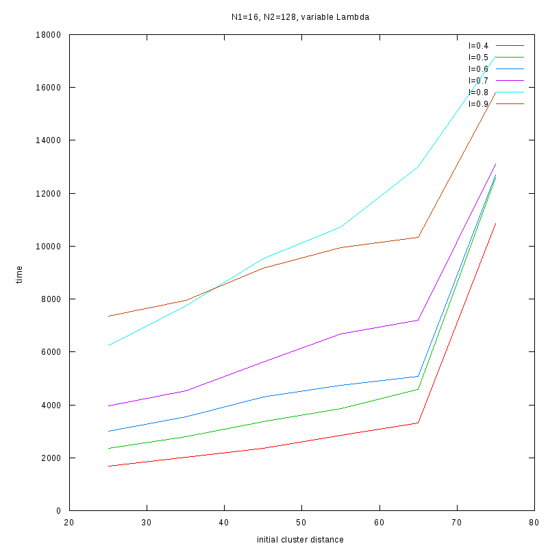
The following two sections show the convergence times for cluster distances
varying from 25 cells to 75 cells with a step of 10 cells where the first cluster always consists
of 16 amoebae, while the size of the second cluster varies from 16 to 160 amoebae with a step
of 16.
The value of
varies from 0.4 to 0.9.
Finally the results are for the same dataset but with two different perspectives,
so that the first considers the same relative cluster sizes for different values of
, while the second considers different cluster sizes for the same value of
In both cases we show the results both as several 2D plots drawn on the same graph
and as a 3D plot with respect to the varying parameter.
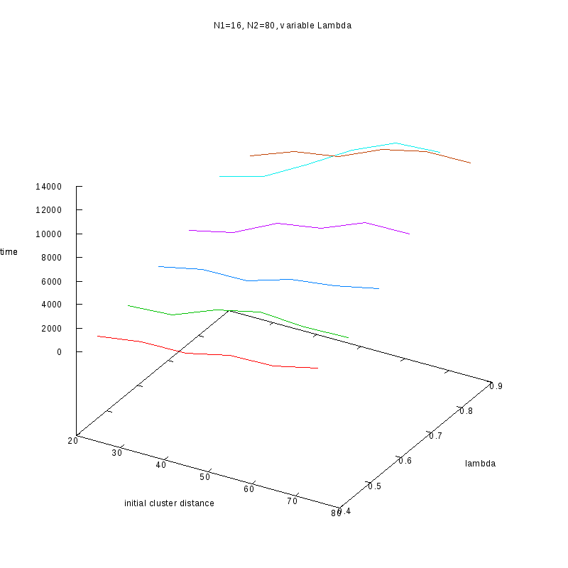
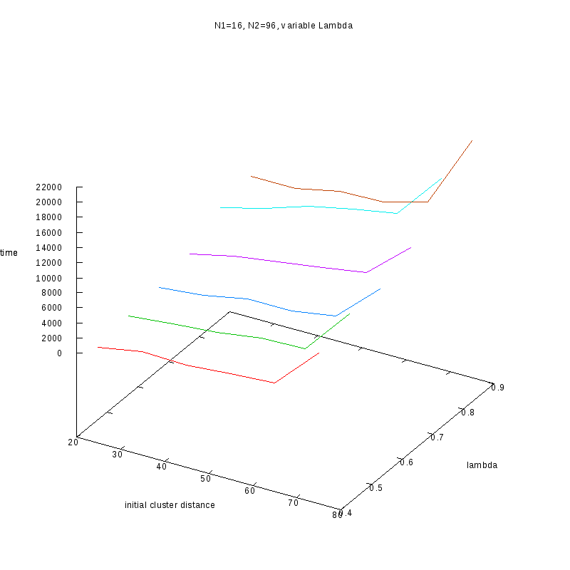
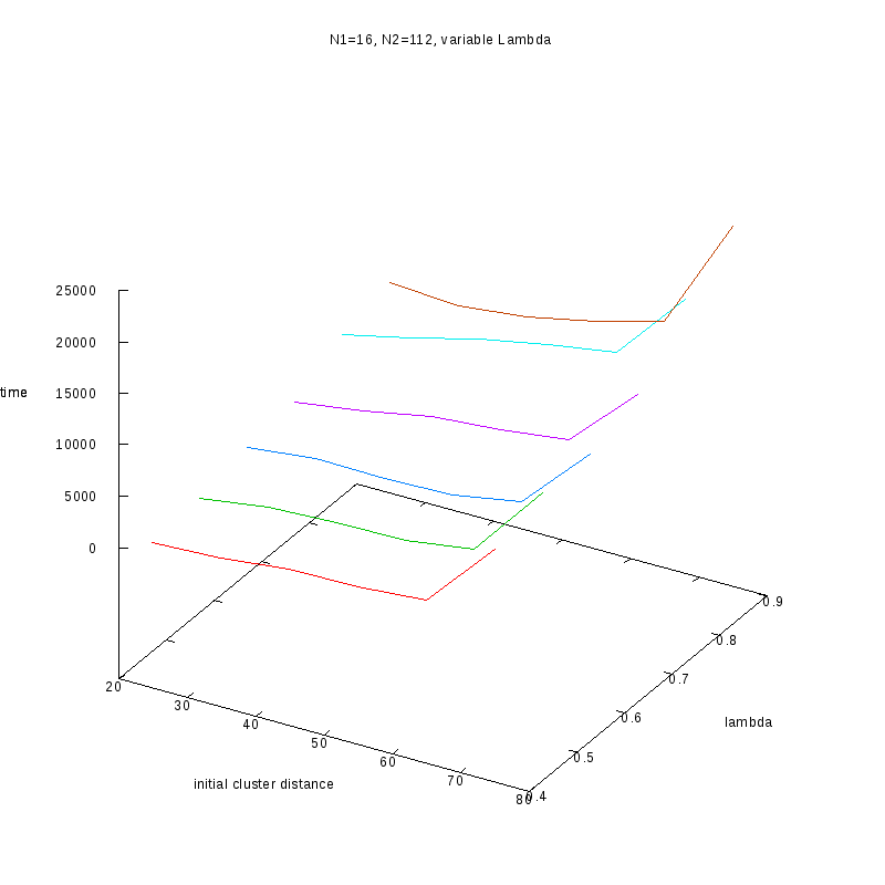
Fixed Cluster Sizes and Variable
The following plots summarize the results for the case where we increase the size of
the second cluster, while keeping
constant.
2D Plots
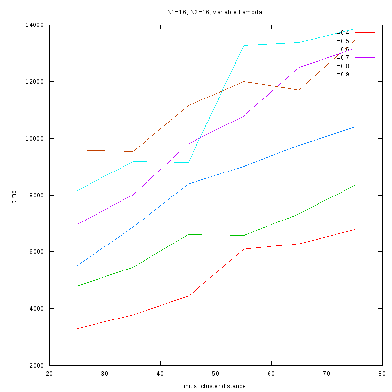
N1=16
N2=16
|
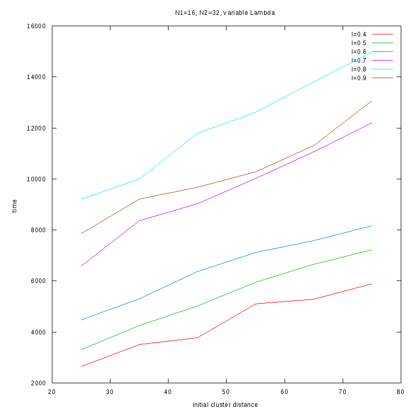
N1=16
N2=32
|
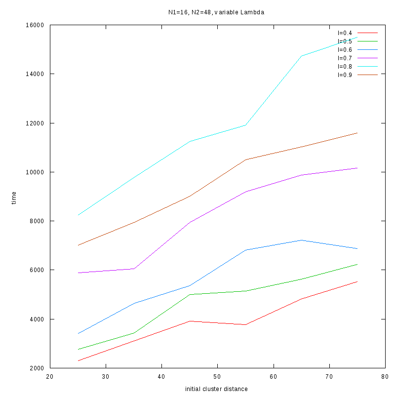
N1=16
N2=48
|
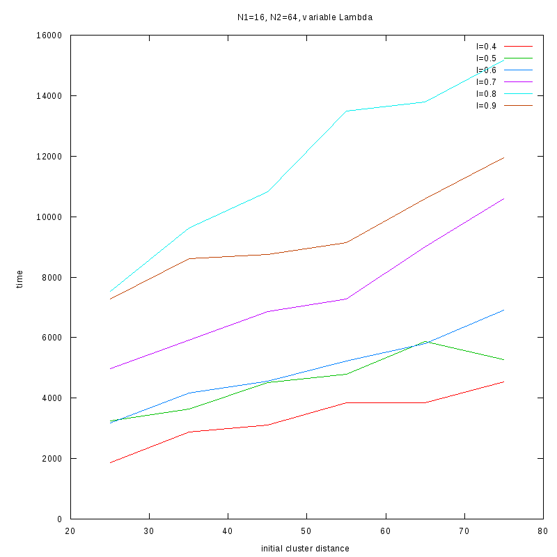
N1=16
N2=64
|
N1=16
N2=80
|
N1=16
N2=96
|
N1=16
N2=112
|
N1=16
N2=128
|
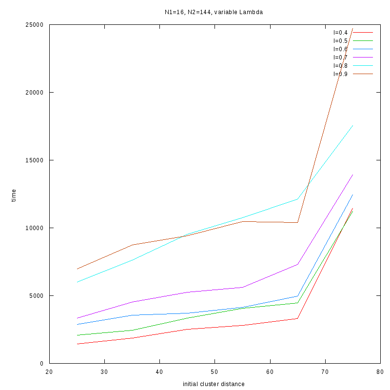
N1=16
N2=144
|
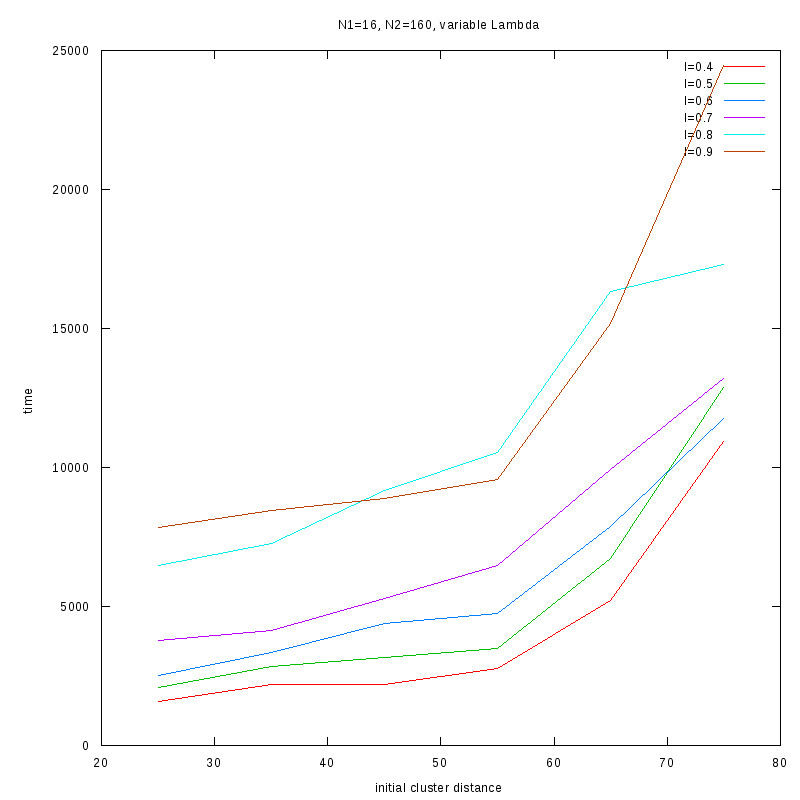
N1=16
N2=160
|
3D Plots
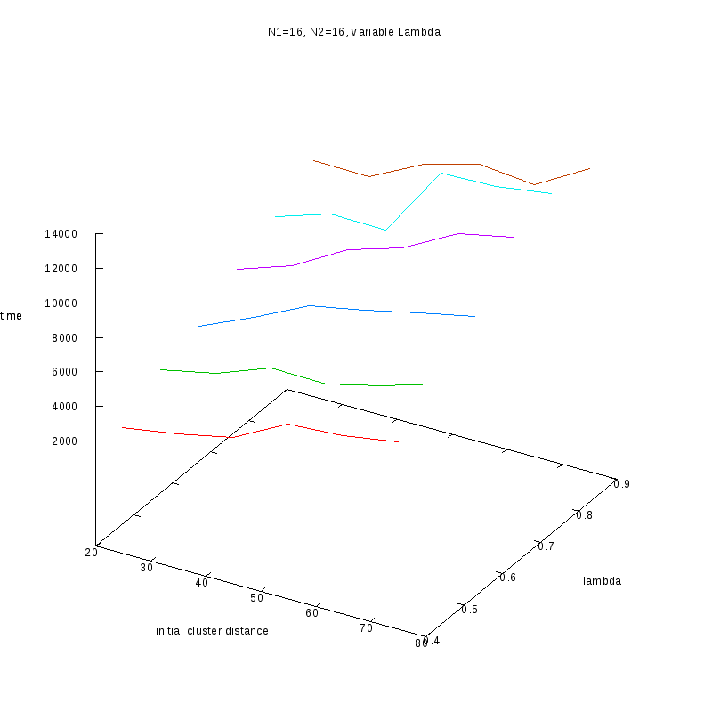
N1=16
N2=16
|

N1=16
N2=32
|
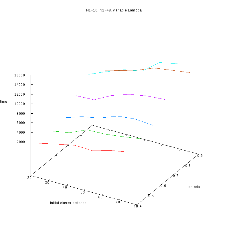
N1=16
N2=48
|
N1=16
N2=64
|
N1=16
N2=80
|
N1=16
N2=96
|
N1=16
N2=112
|
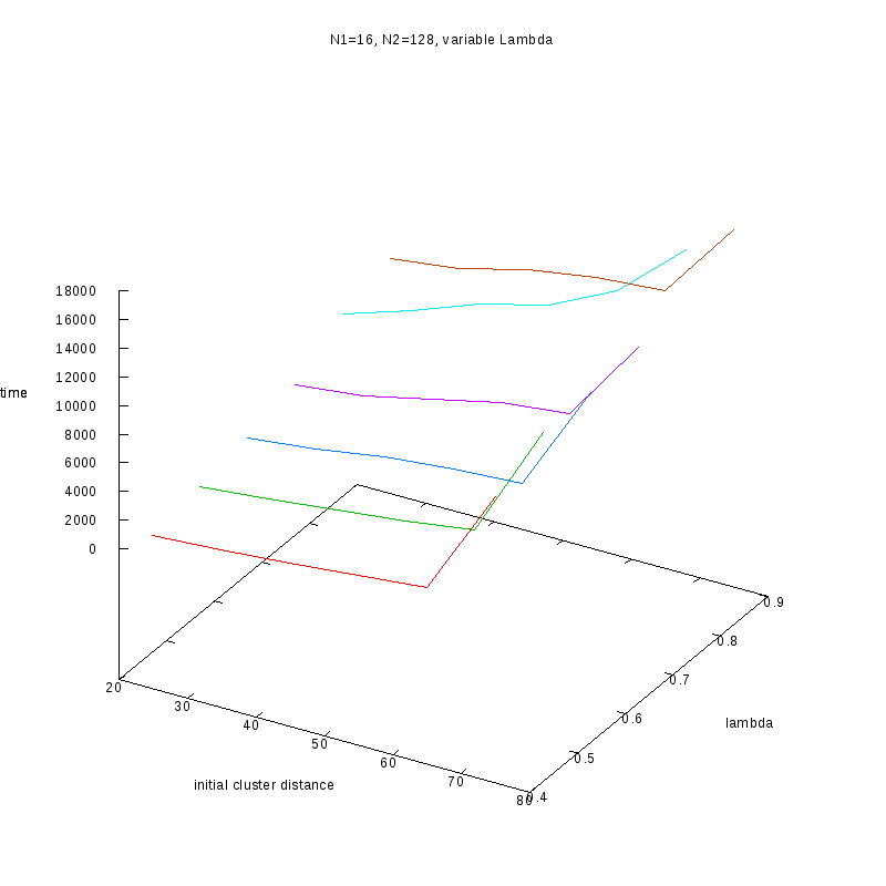
N1=16
N2=128
|

N1=16
N2=144
|
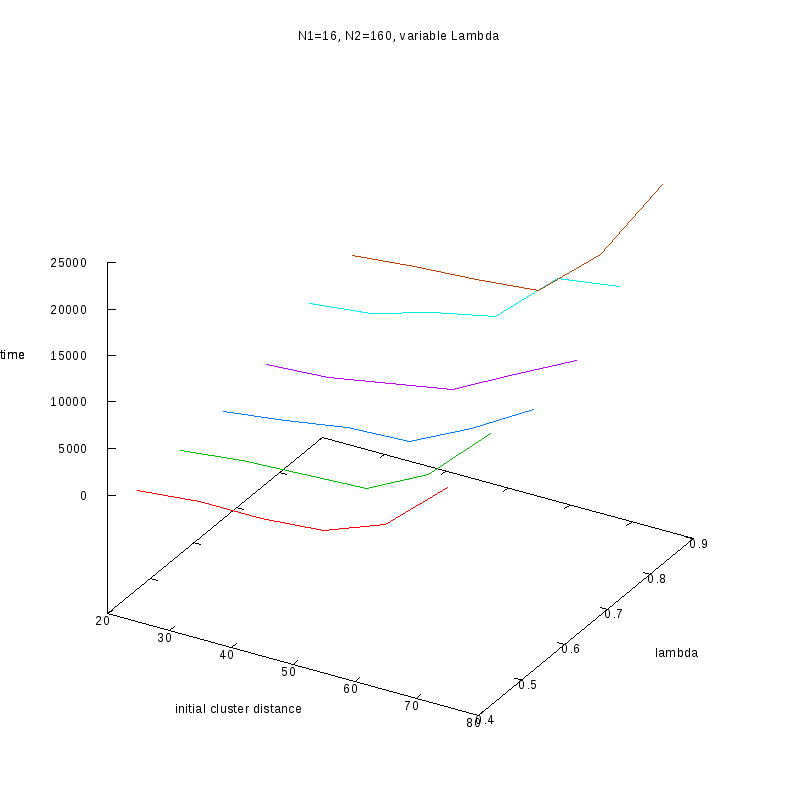
N1=16
N2=160
|
Fixed
and Variable Cluster Sizes
2D Plots
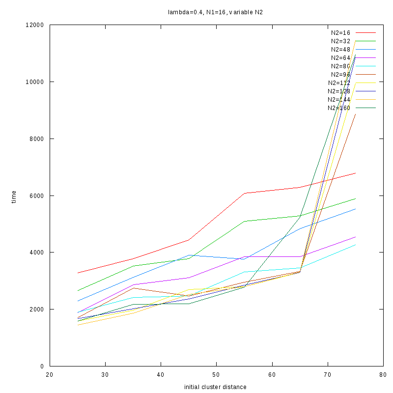
=0.4
|
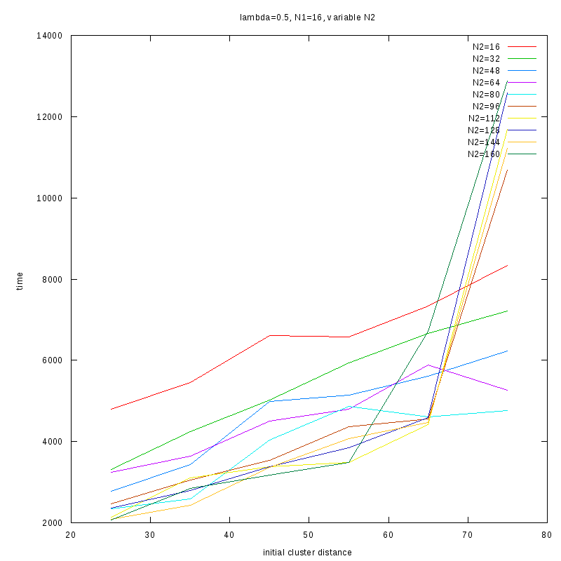
=0.5
|
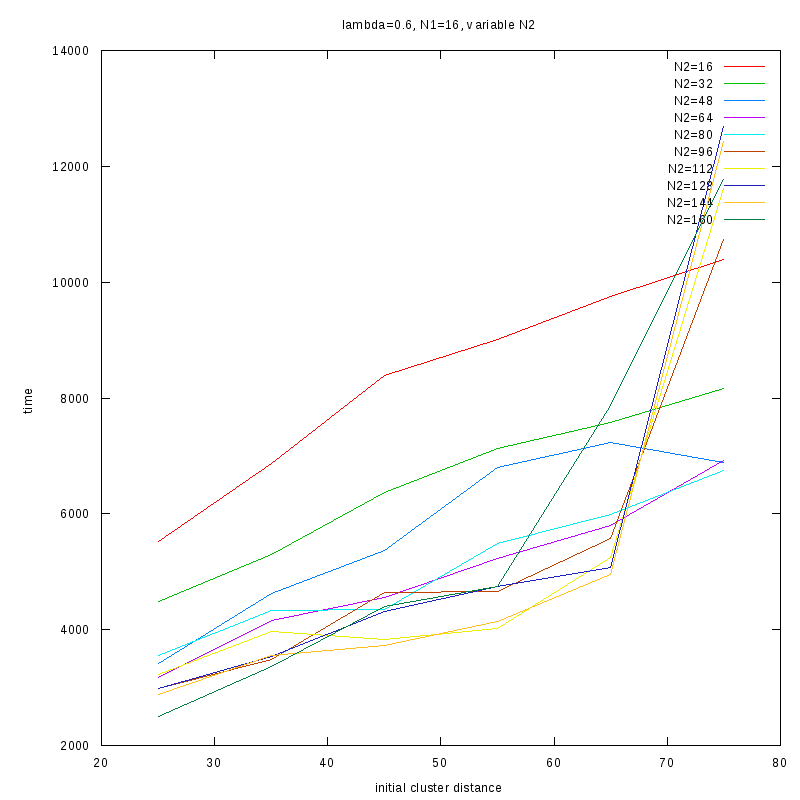
=0.6
|
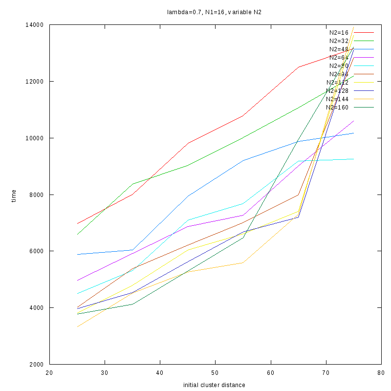
=0.7
|
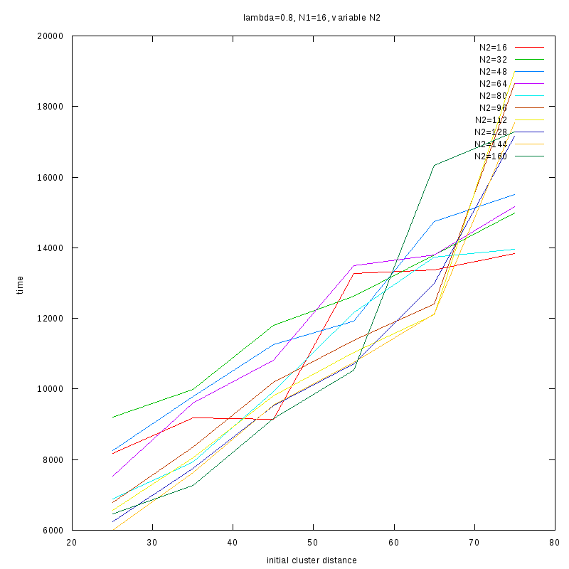
=0.8
|
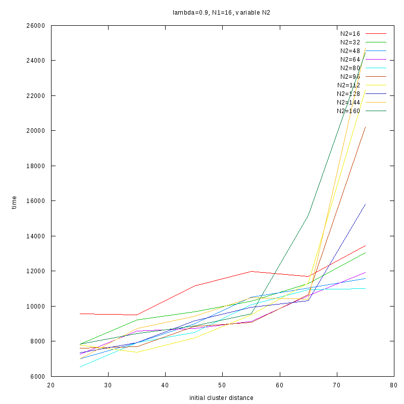
=0.9
|
3D Plots
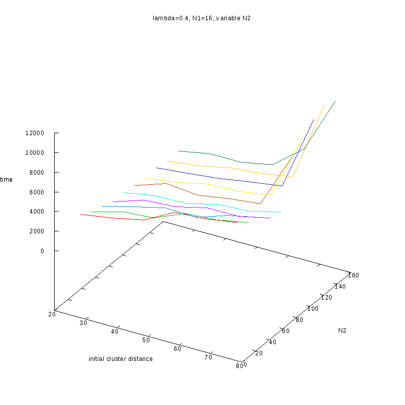
=0.4
|
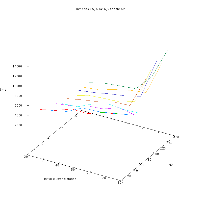
=0.5
|
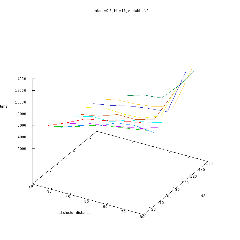
=0.6
|
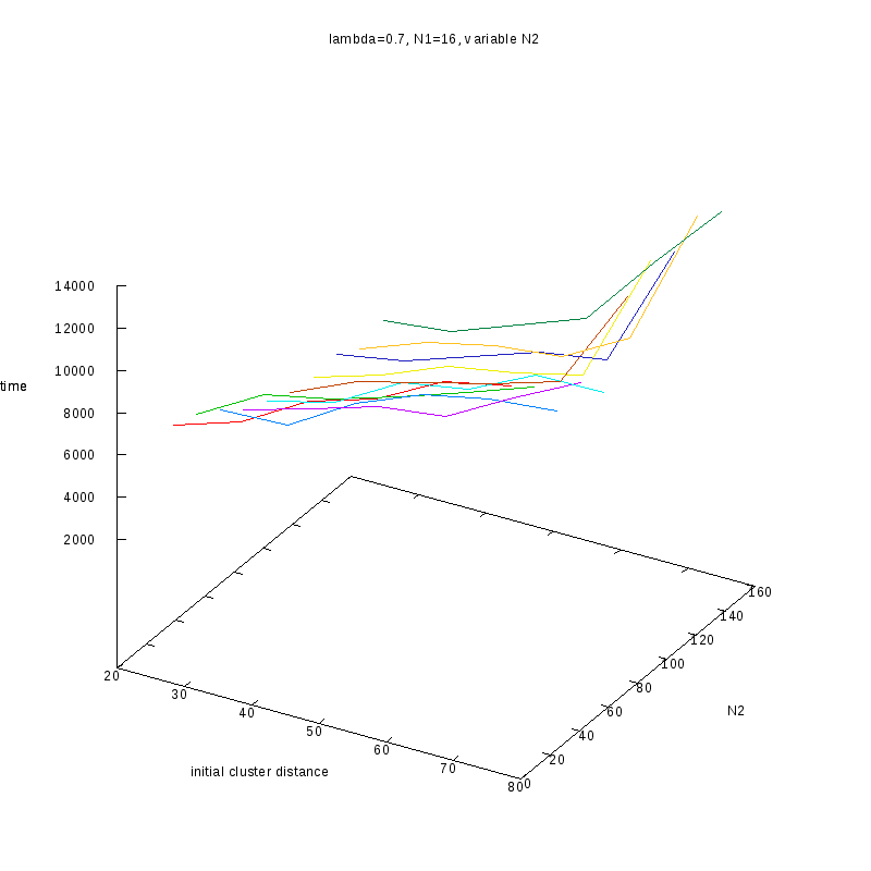
=0.7
|
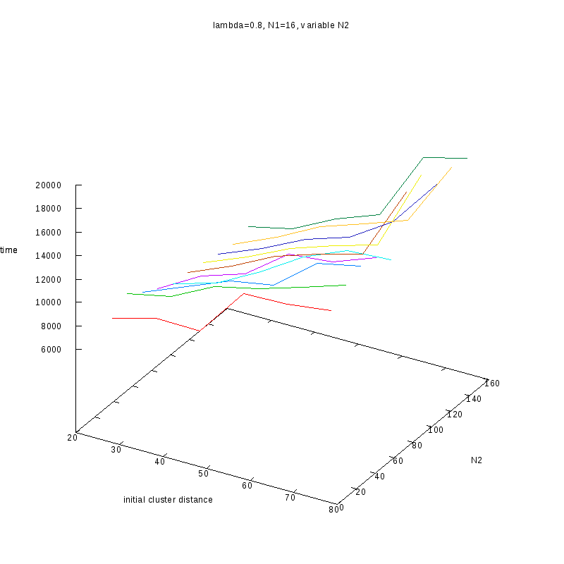
=0.8
|
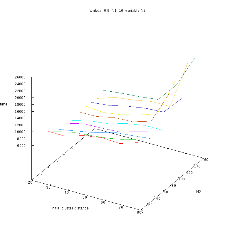
=0.9
|
Comments on the above results
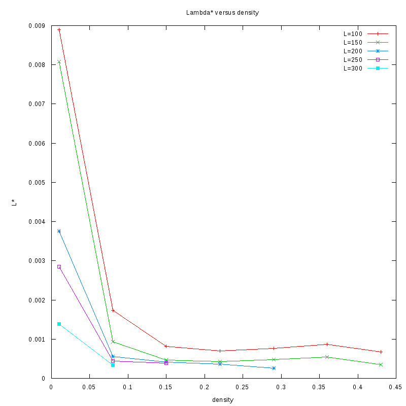
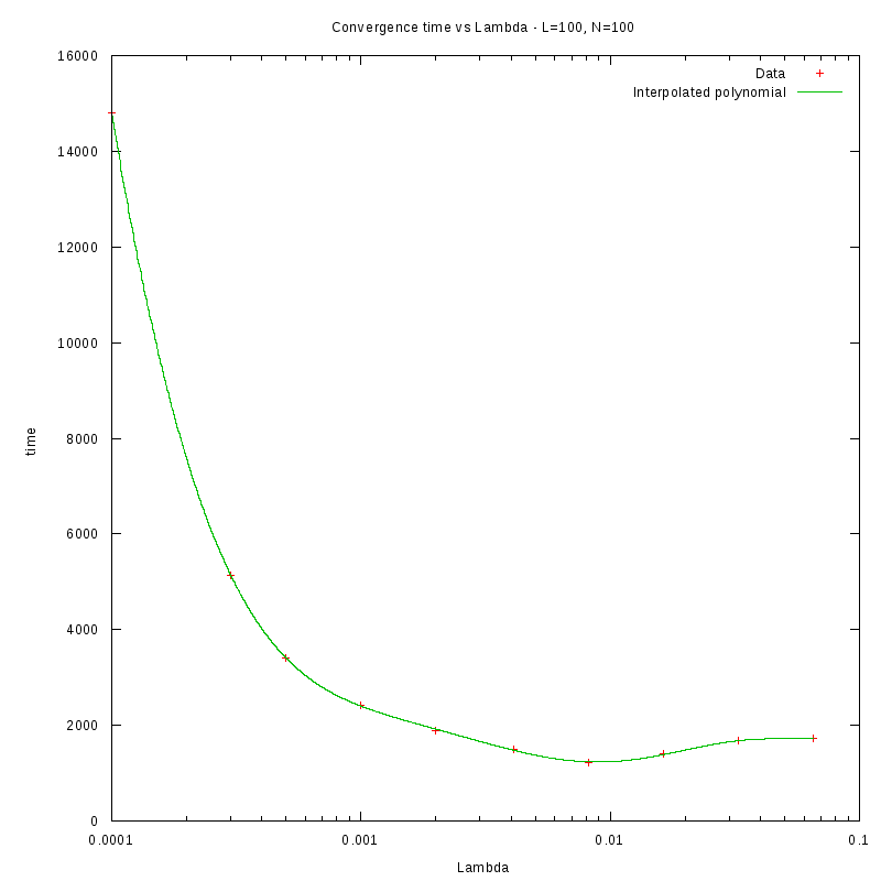
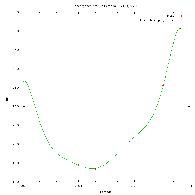
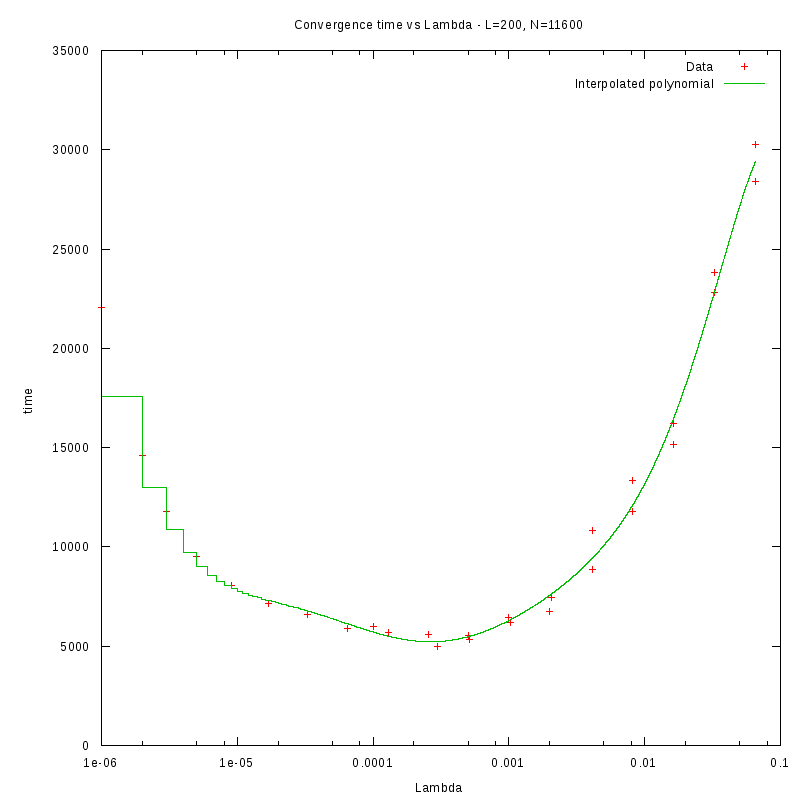
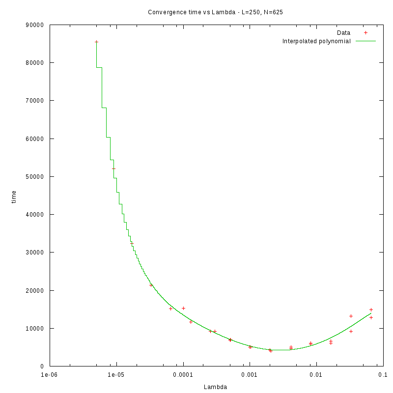
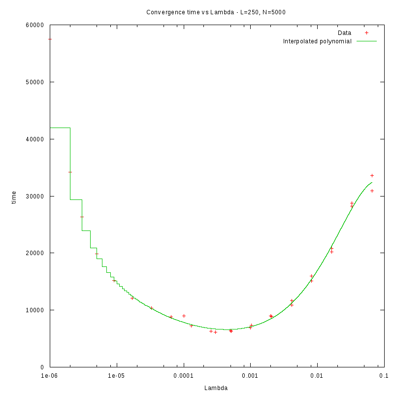
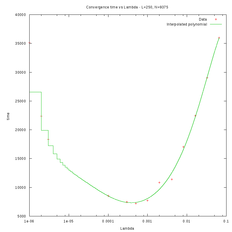
Results on the optimal fire rate
In this subsection we present some results regarding how the optimal fire rate,
, varies with
respect to the density and grid size or grid size and number of amoebae N.
Our observations so far indicate that the value of
could be, in the general sense,
“configuration“ dependent, i.e. not only it varies with respect to L and N, but also
with respect to the current configuration of the amoebae (such first indications are due to our
experiments with 2 amoebae).
Nevertheless, these experiments try to measure the “mean (w.r.t. configurations) optimal
“
given the grid size and number of amoebae.
Finally, we try to deduce some empirical relation that will help identify approximately the value of
given N and L.
Density and environment size
L=100
d=01%
|
N=100
d=08%
|
L=100
d=15%
|
L=100
d=22%
|
N=100
d=29%
|
L=100
d=36%
|
L=100
d=43%
|
L=150
d=01%
|
L=150
d=08%
|
L=150
d=15%
|
L=150
d=22%
|
L=150
d=29%
|
L=150
d=36%
|
L=150
d=43%
|
L=200
d=01%
|
L=200
d=08%
|
L=200
d=15%
|
L=200
d=22%
|
L=200
d=29%
|
L=250
d=01%
|
L=250
d=08%
|
L=250
d=15%
|
N=300
d=01%
|
N=300
d=08%
|
as a function of density for different N
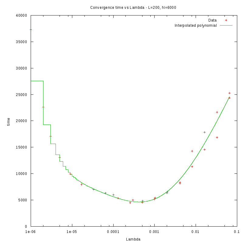
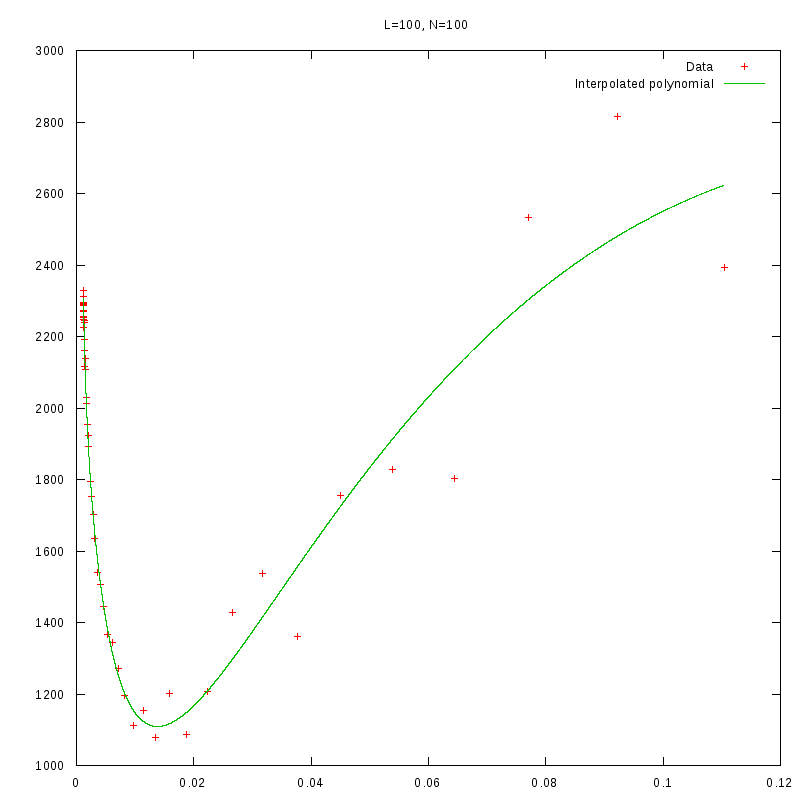
Environment size and Number of amoebae
Having identified some first approximations on the values of
with respect
to the density and the environment size, we were able to perform more detailed
experiments that were focused closer to the
value.
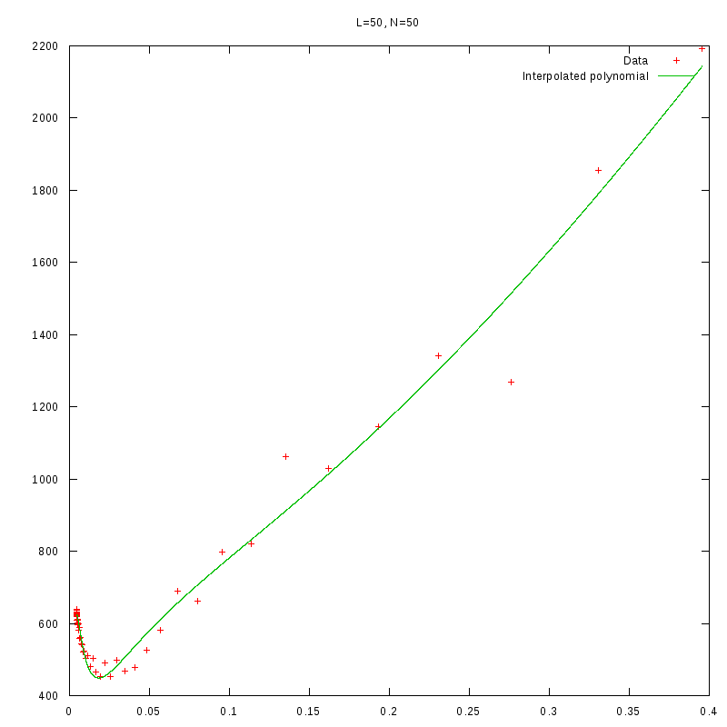
L=50
N=50
|
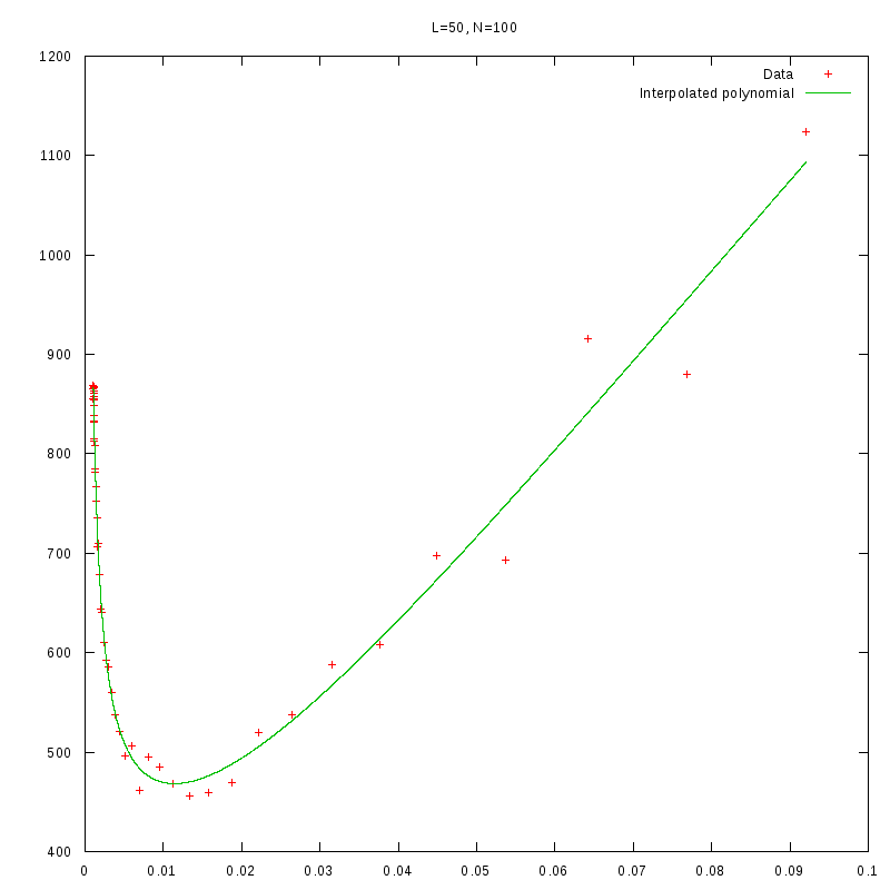
L=50
N=100
|
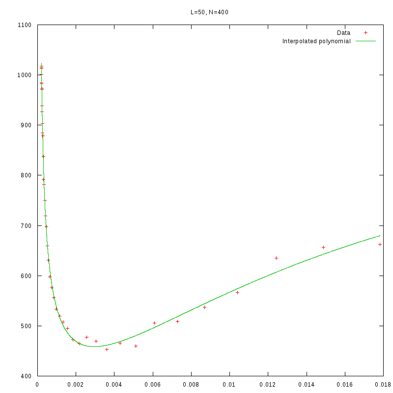
L=50
N=400
|
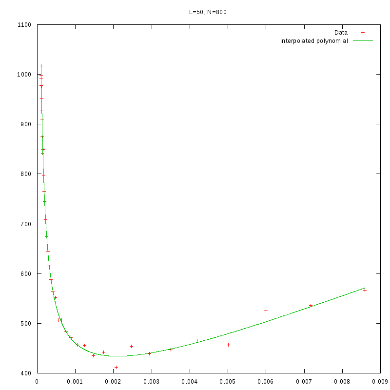
L=50
N=800
|
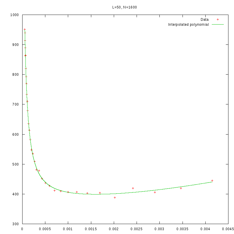
L=50
N=1600
|
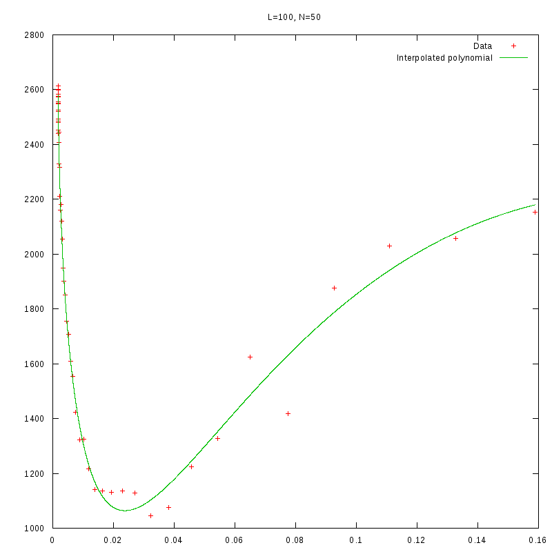
L=100
N=50
|
L=100
N=100
|
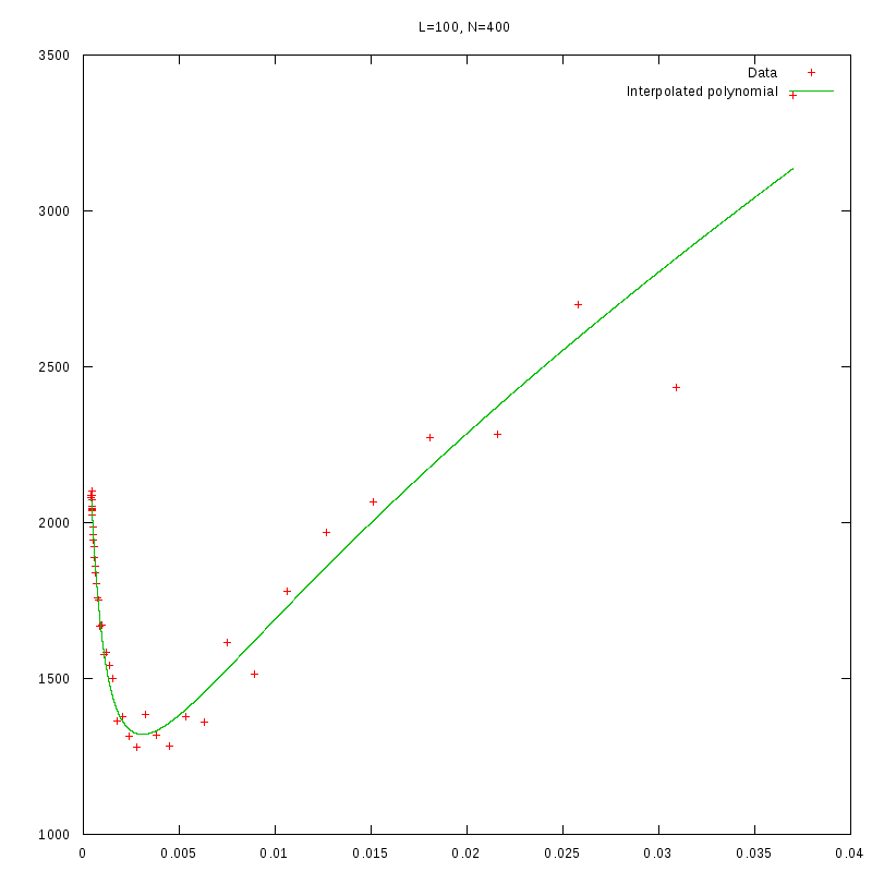
L=100
N=400
|
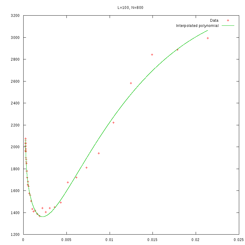
L=100
N=800
|
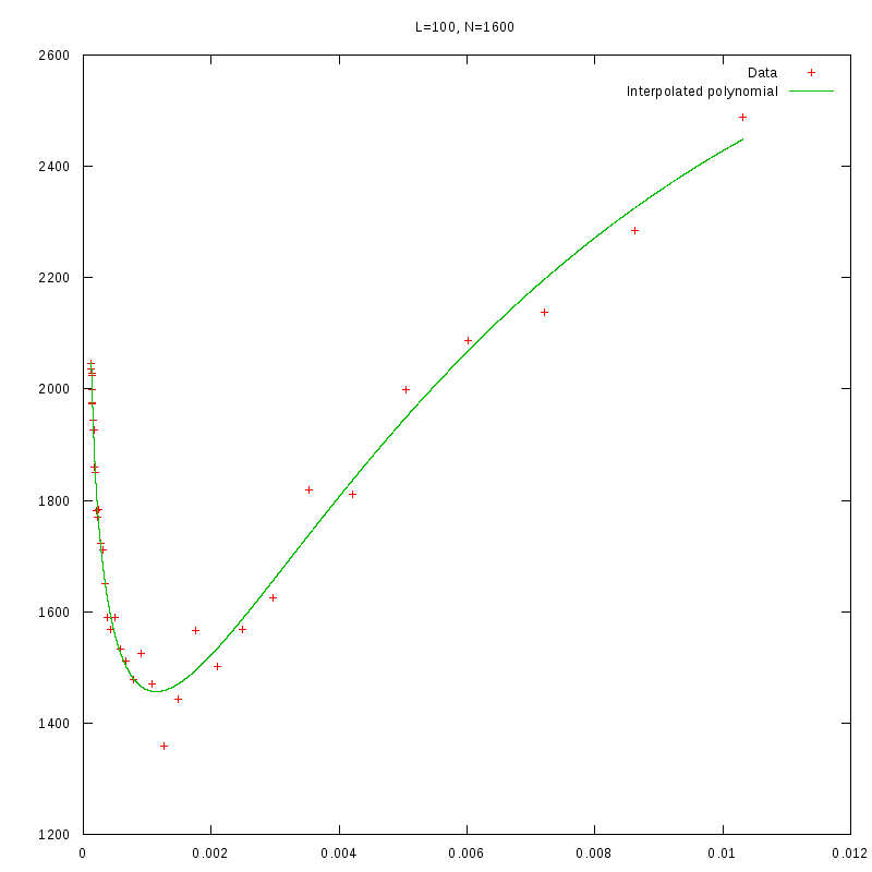
L=100
N=1600
|
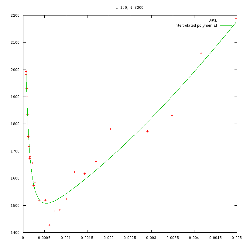
L=100
N=3200
|
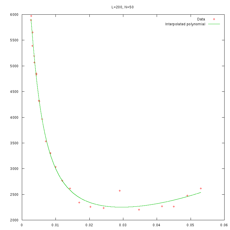
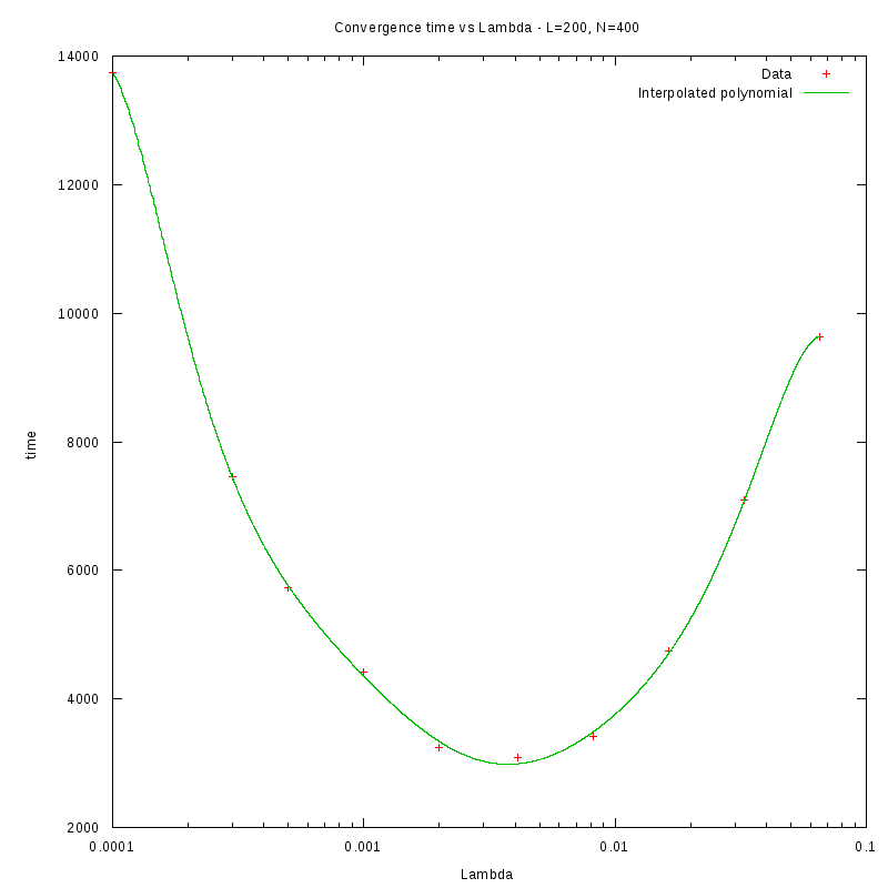
L=200
N=50
|
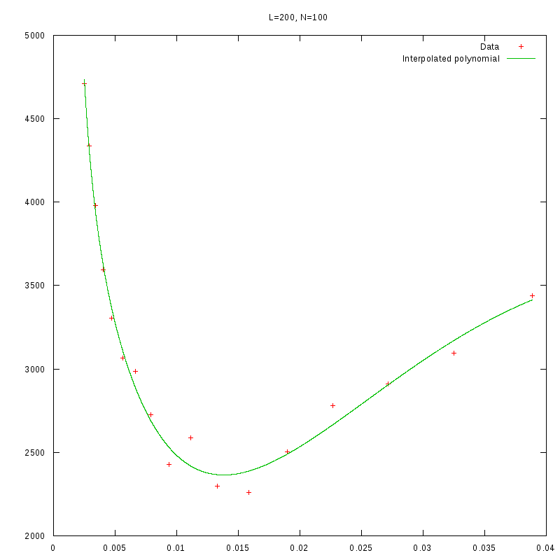
L=200
N=100
|
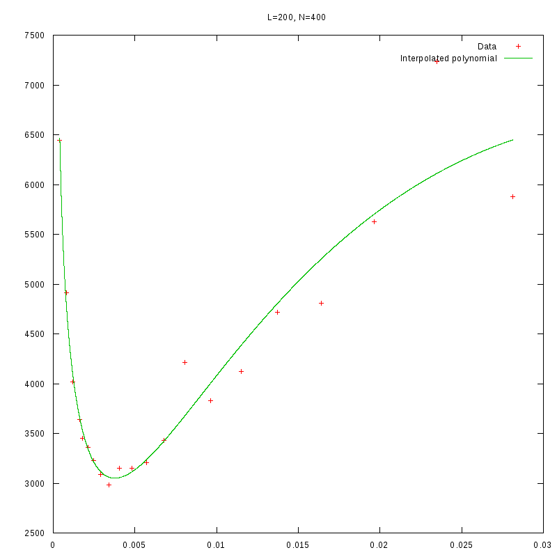
L=200
N=400
|
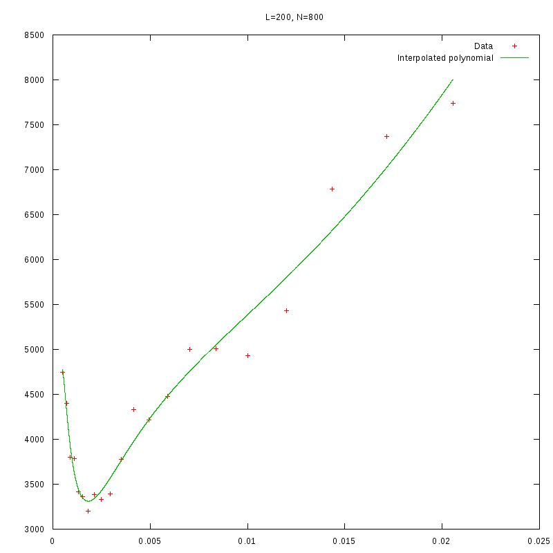
L=200
N=800
|
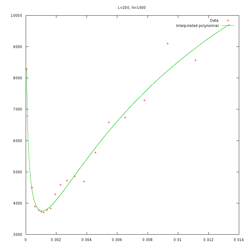
L=200
N=1600
|
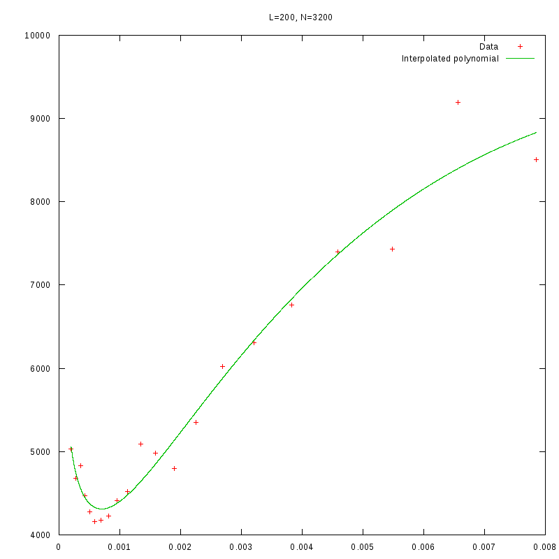
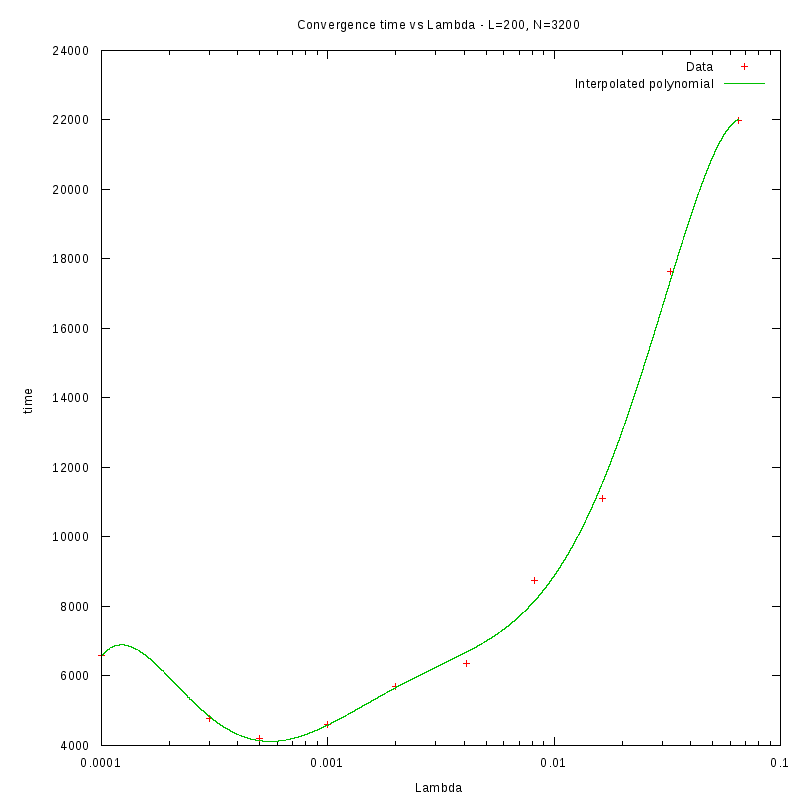
L=200
N=3200
|
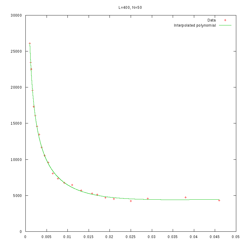
L=400
N=50
|
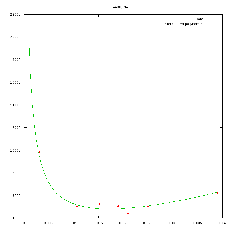
L=400
N=100
|
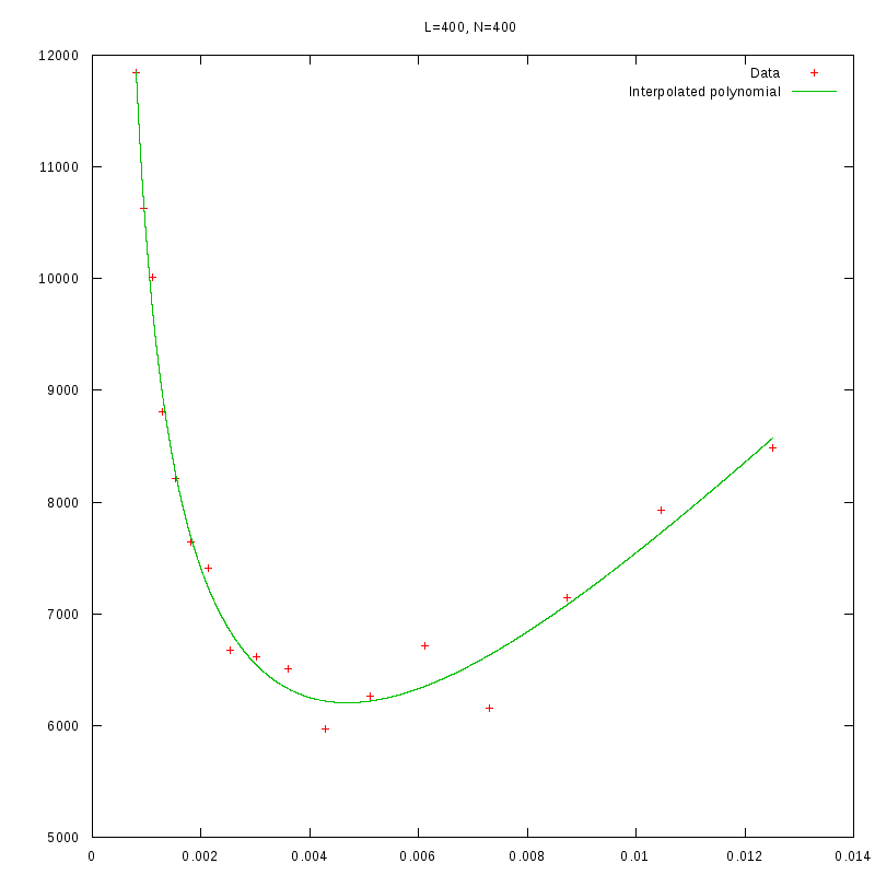
L=400
N=400
|
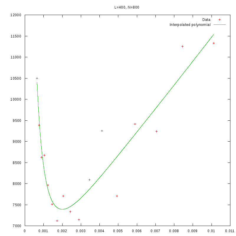
L=400
N=800
|
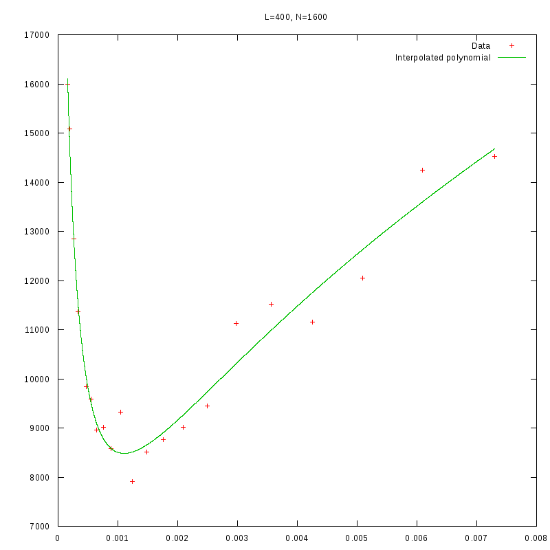
L=400
N=1600
|
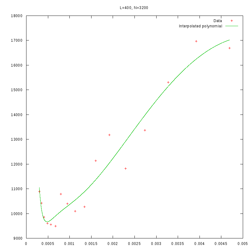
L=400
N=3200
|
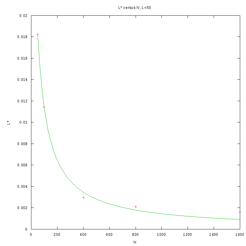
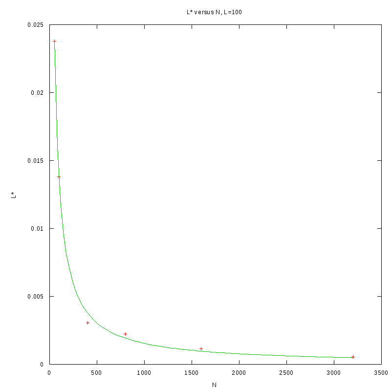
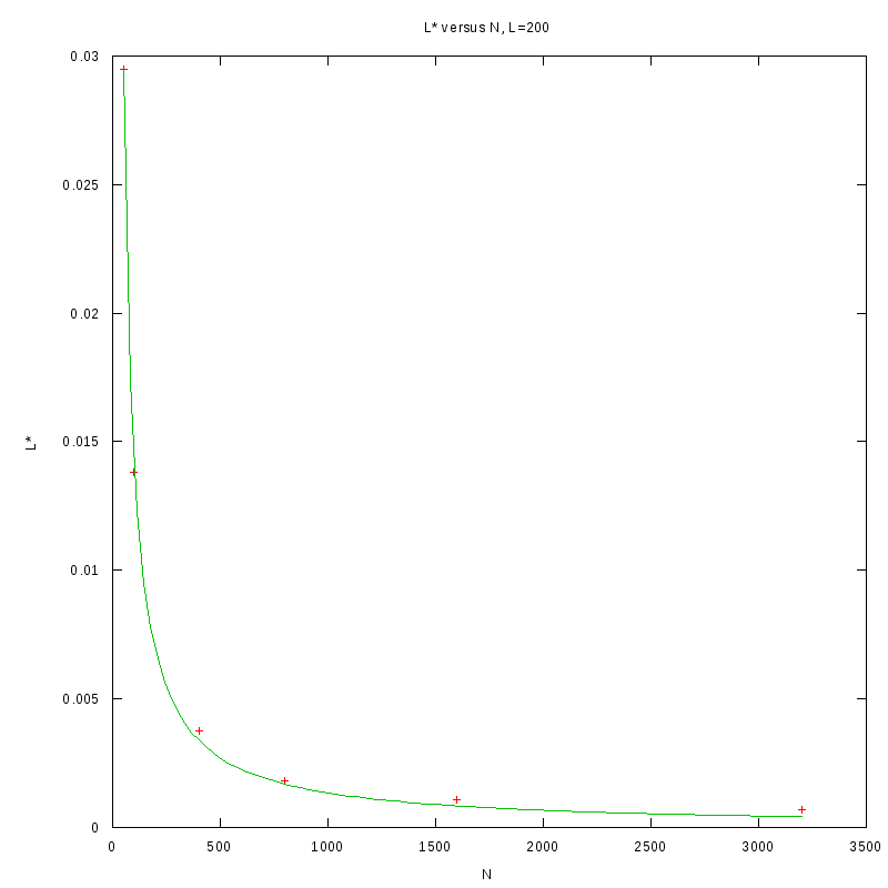
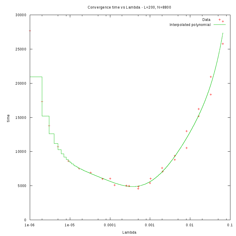
versus N
An empirical relationship for
as a function of L
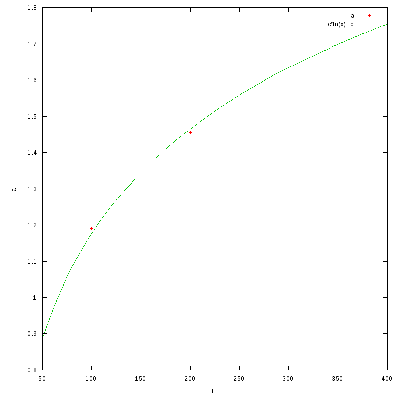
As we observe from our results, for each value of L,
is inversely proportional
to N.
By fitting the experimental values to a curve of the form
 we obtain the following results
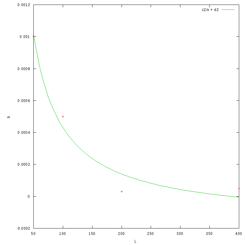
| L | a | b |
| 50 | 0.88(0.05) | 0.001(0.0005) |
| 100 | 1.19(0.04) | 0.0005(0.0004) |
| 200 | 1.455(0.026) | 0.00003(0.0002) |
| 400 | 1.757(0.016) | 0.00005(0.00014) |
The following image shows a plot of the a coefficient as a function of L,
as well as an fit to the function
 The corresponding coefficients for this function are
| c | d |
0.418(0.008) | -0.75(0.04) |
Similarly, the following image shows a fit of the b coefficient of the above relationship
to a curve of the form
 with coefficients
| c2 | d2 |
0.058(0.007) | -0.00015(0.00009) |
Combining the above relations we find the following
empirical approximation for
as a function of L, N:
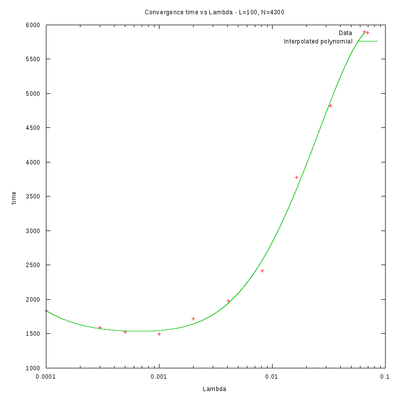
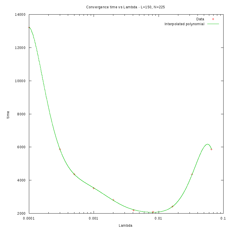
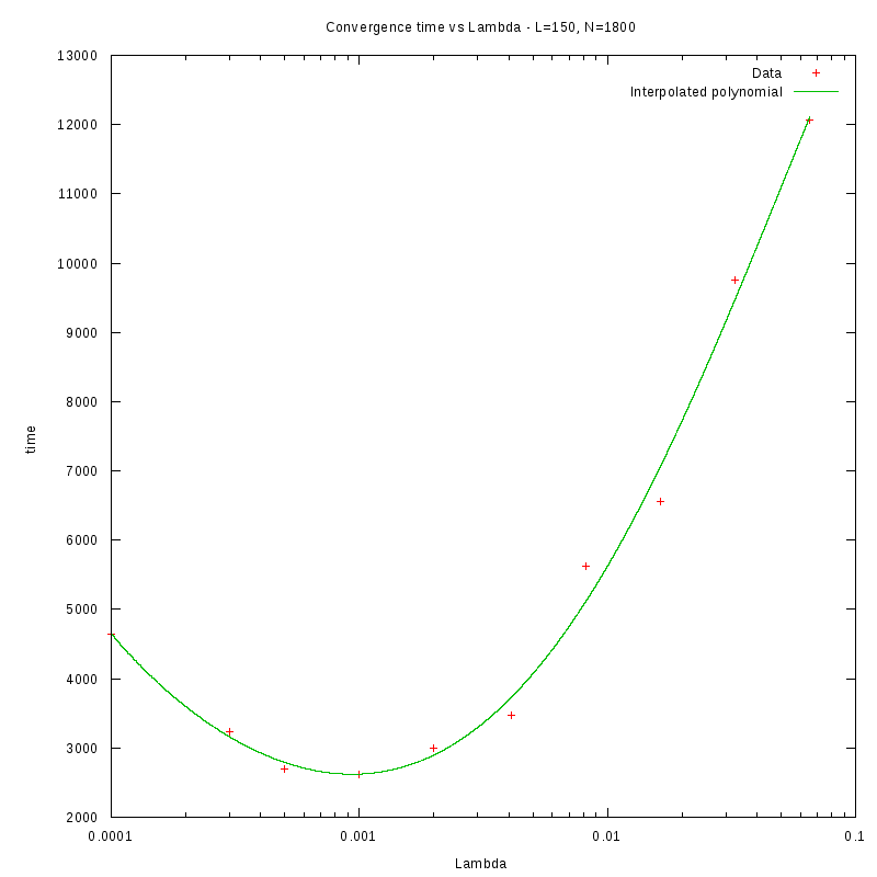
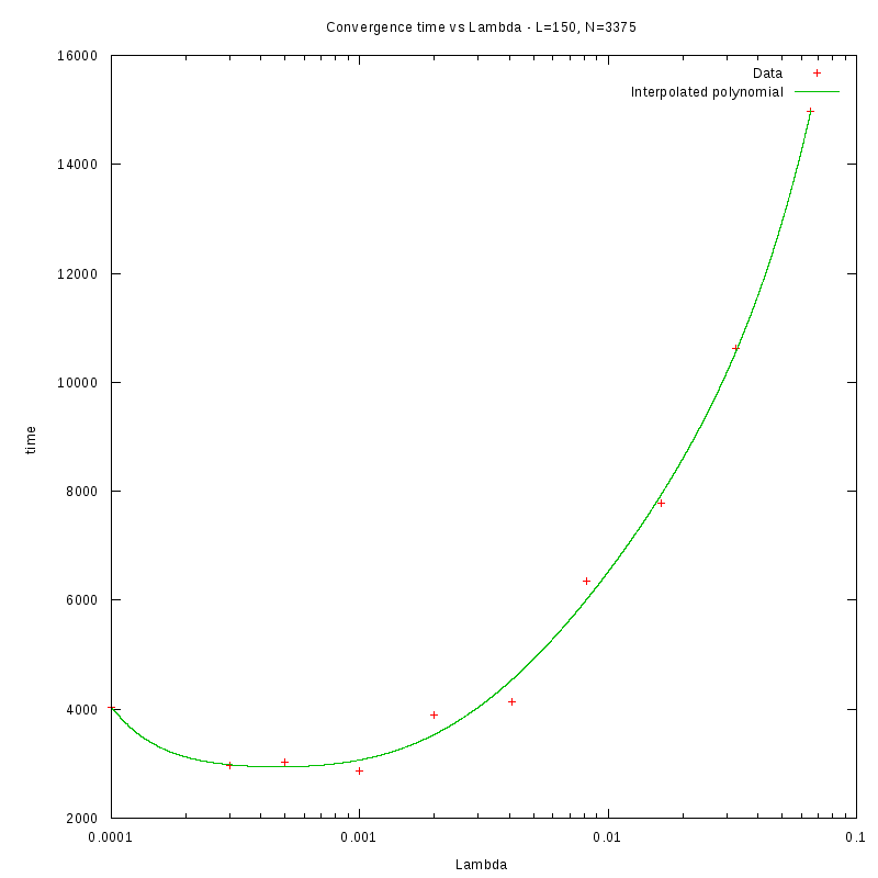
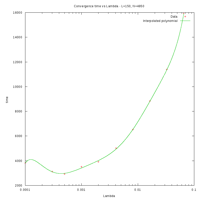
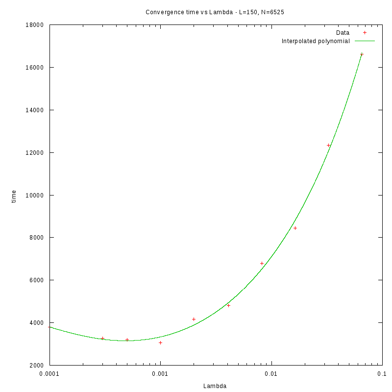
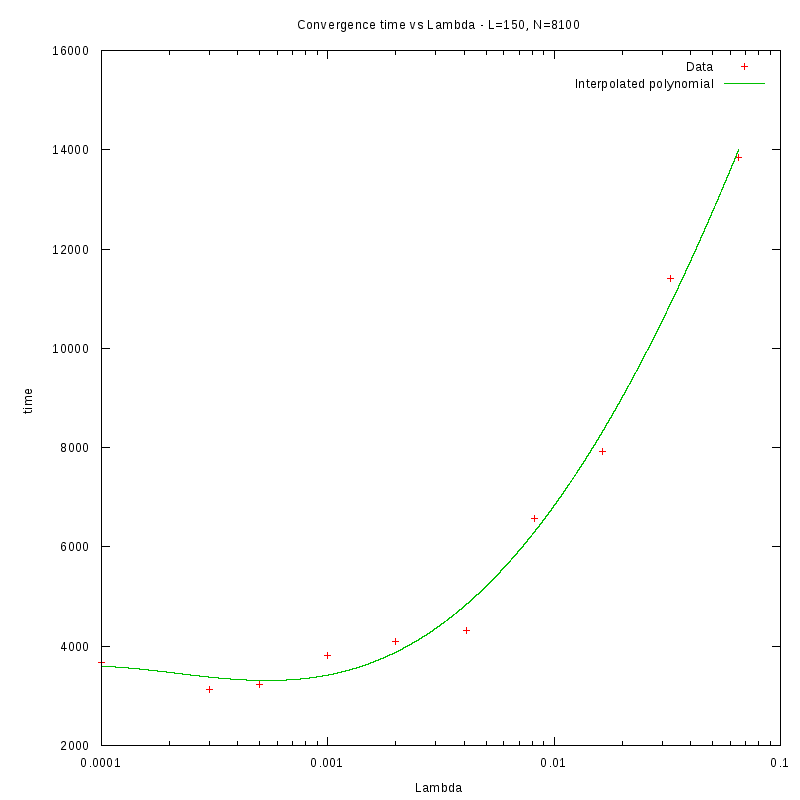
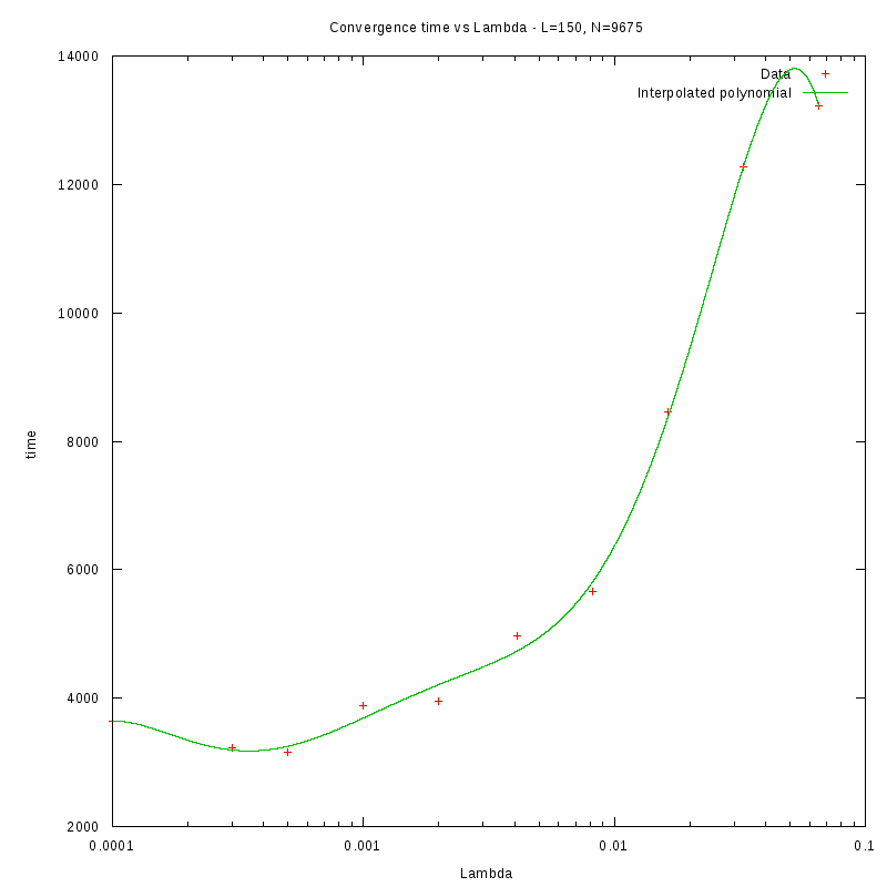
 As a quick verification, we applied the above formula in the results of the previous section, where we
calculated
as a function of density.
The images below show that the empirical relation is in good accordance with the experimental data,
although this is something we expected, since the values of L and N are within the range of the values
that were used to generate the relation.
As a quick verification, we applied the above formula in the results of the previous section, where we
calculated
as a function of density.
The images below show that the empirical relation is in good accordance with the experimental data,
although this is something we expected, since the values of L and N are within the range of the values
that were used to generate the relation.
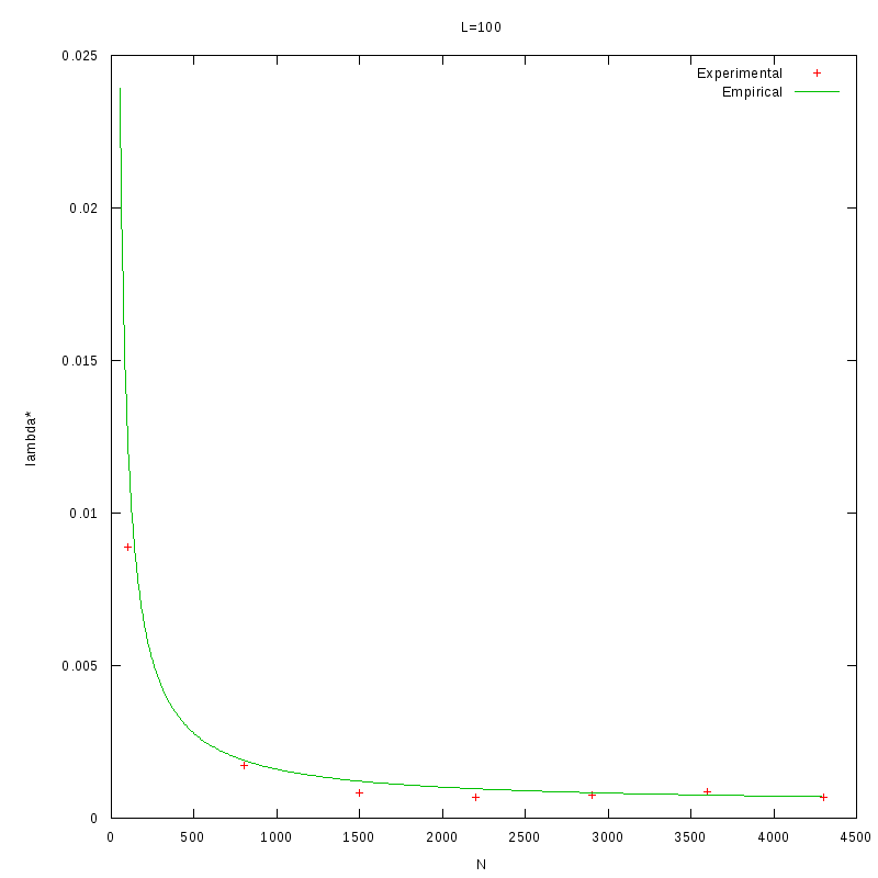
L=100 verification
|
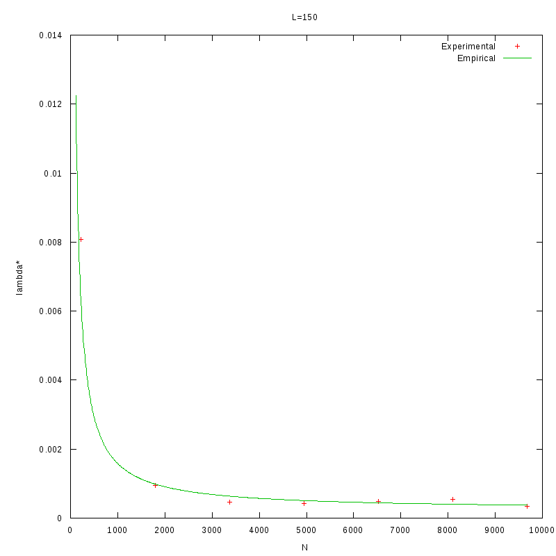
L=150 verification
|
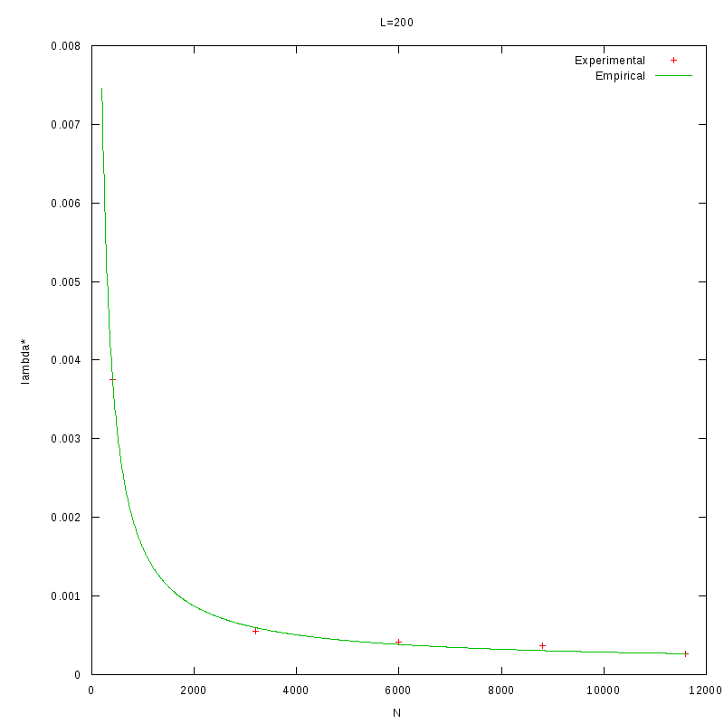
L=200 verification
|
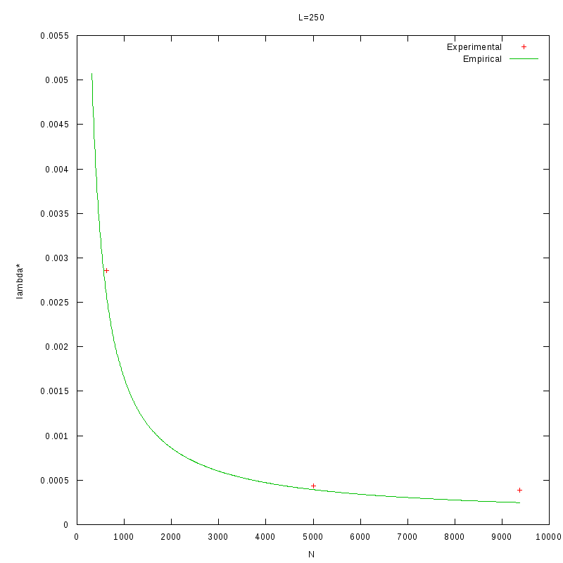
L=250 verification
|
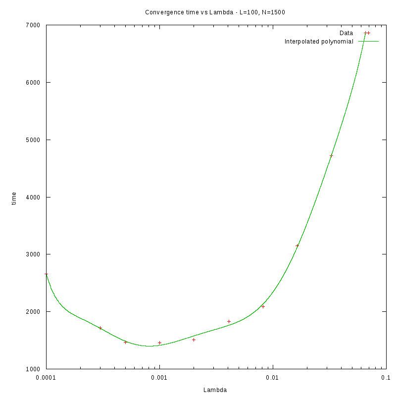
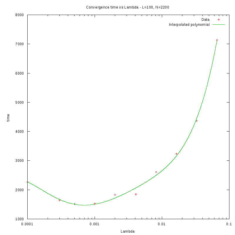
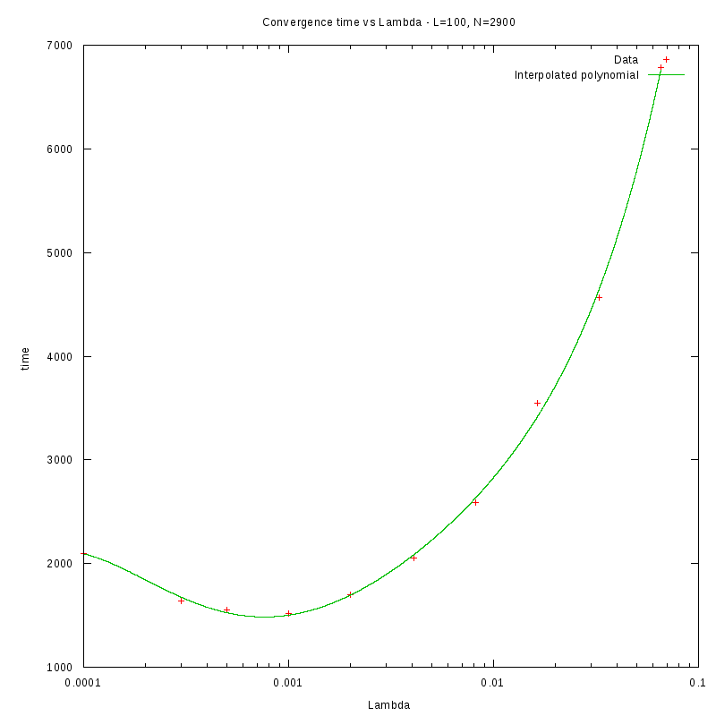
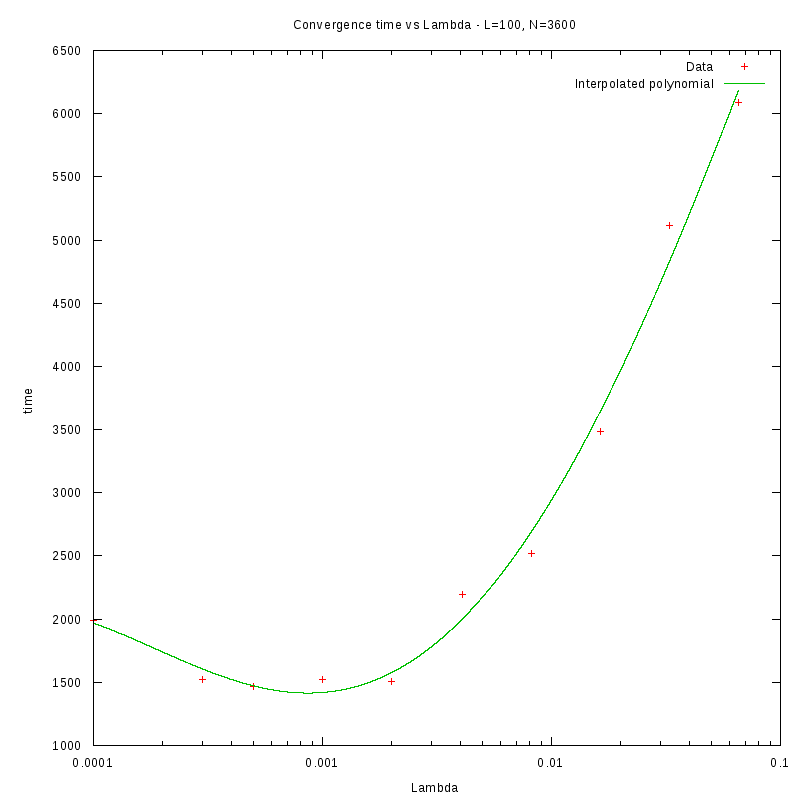
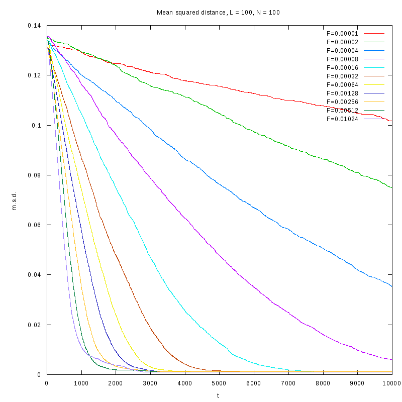
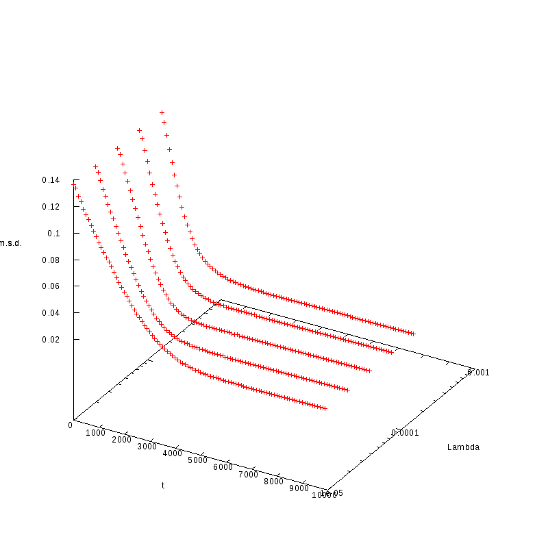
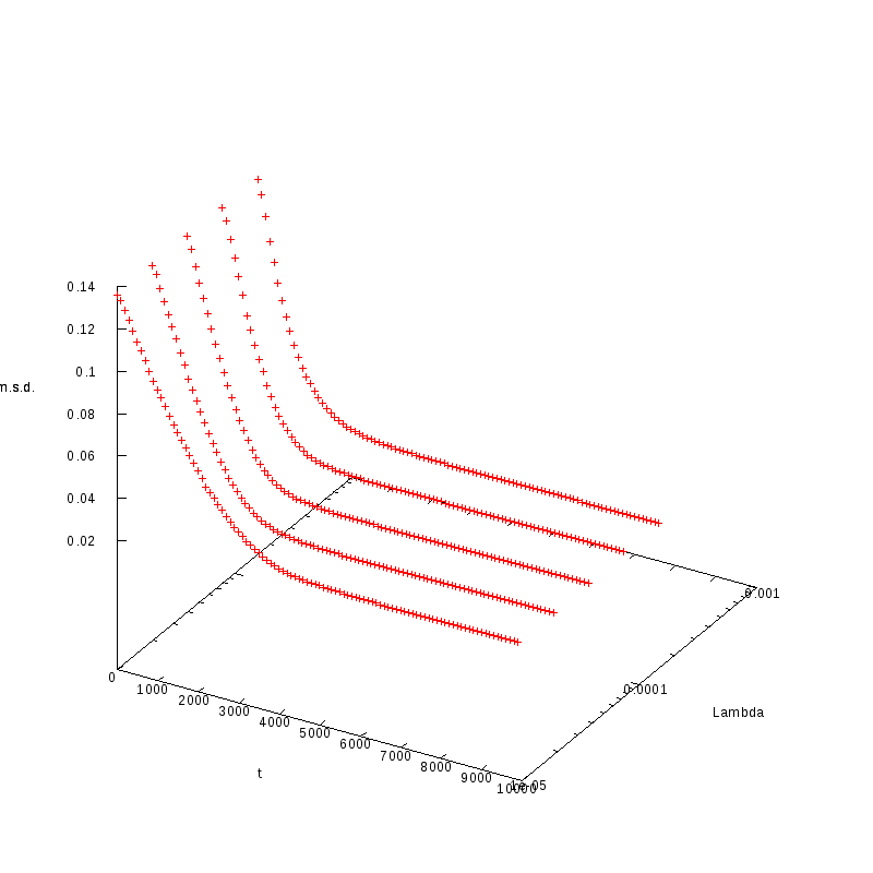
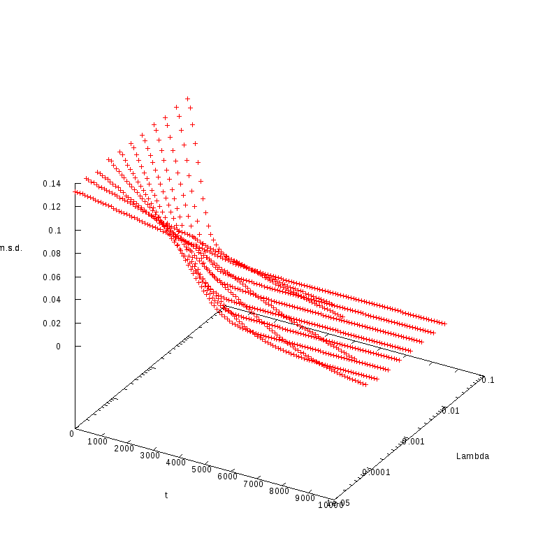
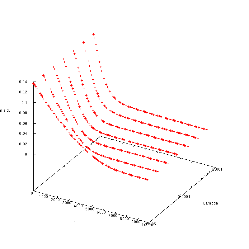
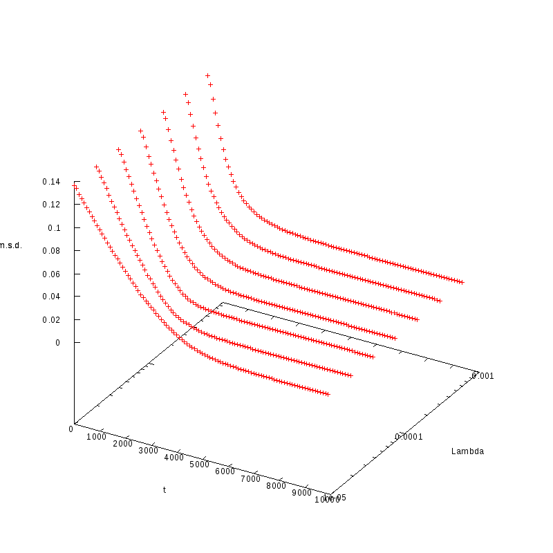
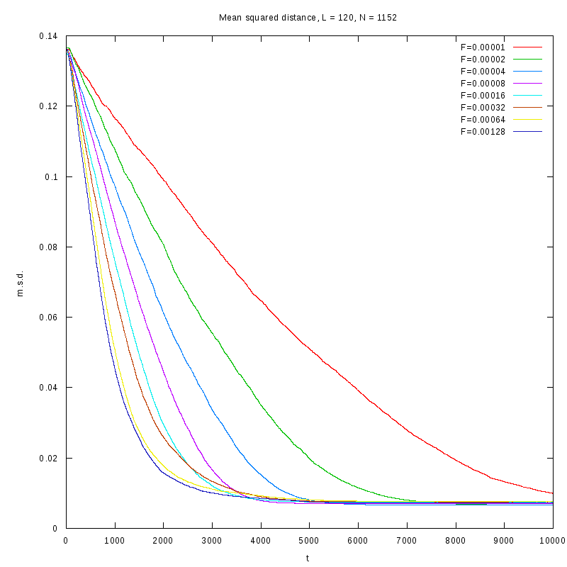
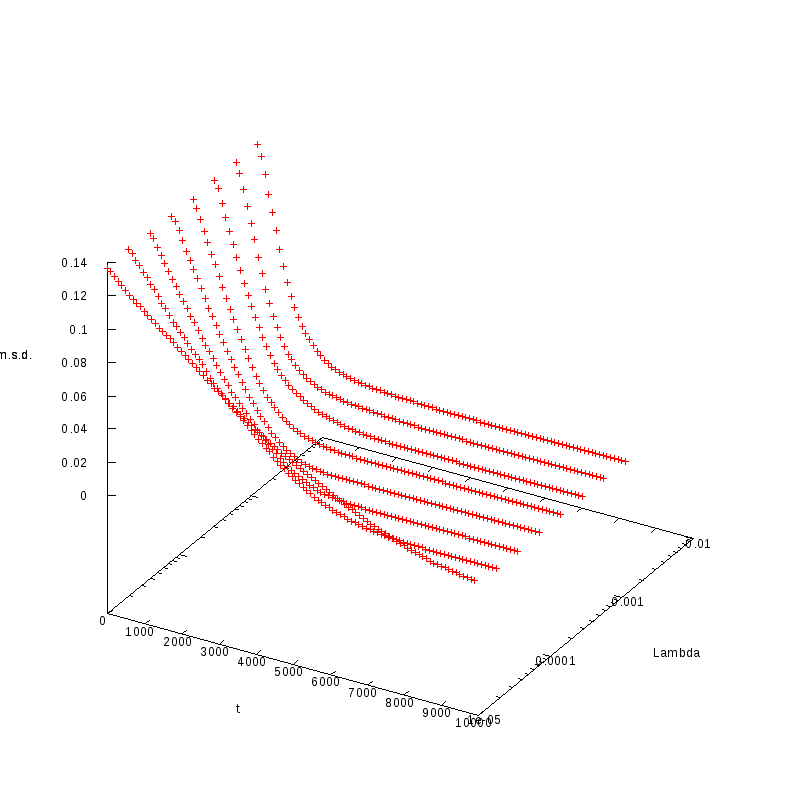
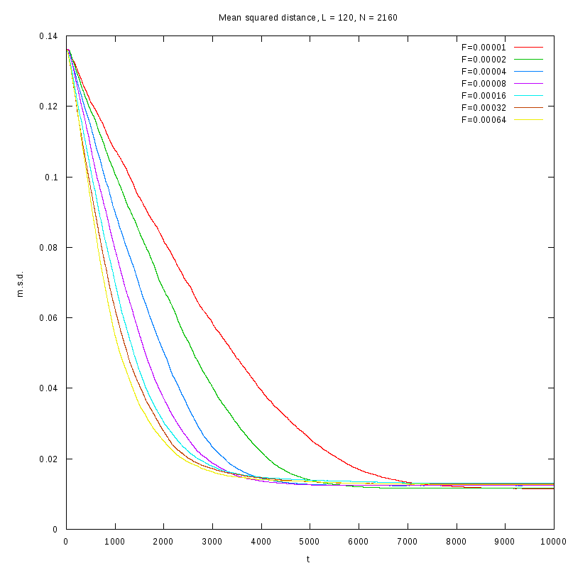
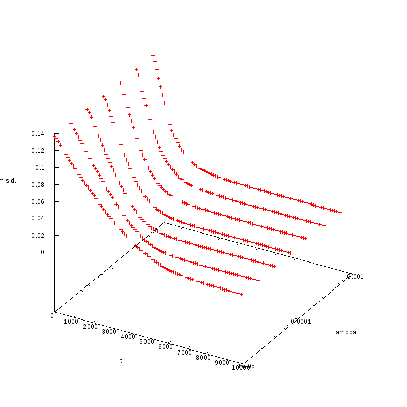
Normalized Mean Square Distance
The purpose of these experiments was to identify how the normalized mean squared distance
varies with respect to the time for different values of
Let di, j denote the distance of amoebae i and j respectively, if this distance
is taken to be normalized, i.e. the respective coordinates
ix
,
iy
,
jx
,
jy
are divided by the environment dimensions.
Further, let the number of agents be
NA
, then the measured quantity is
 where
where
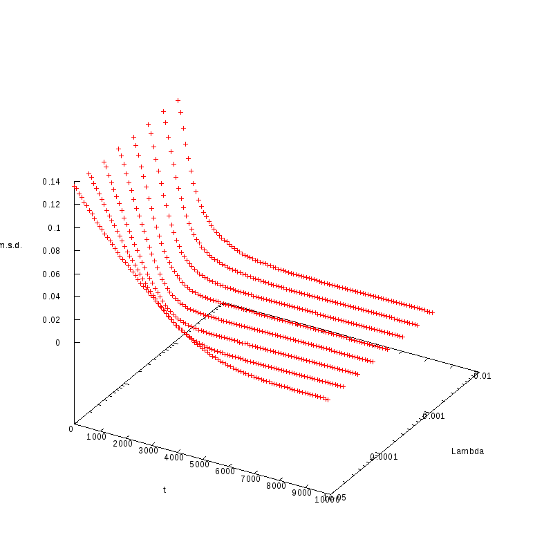
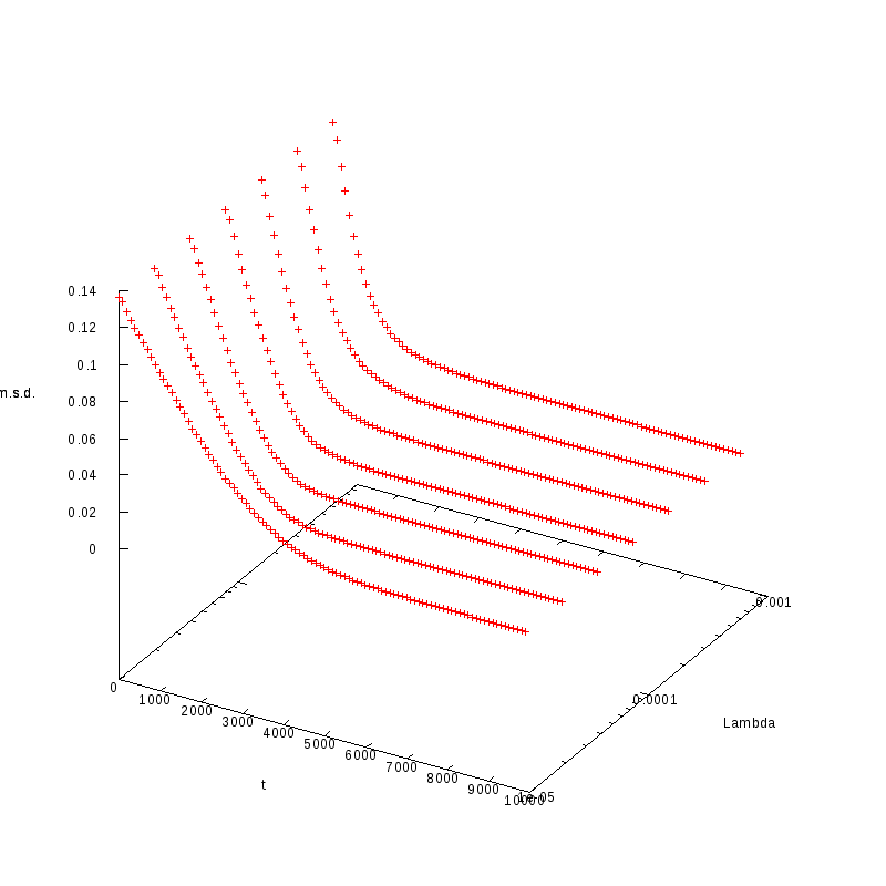
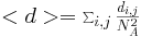 The measurements have been taken for L = 100, 110, 120 and densities ranging from 1% to
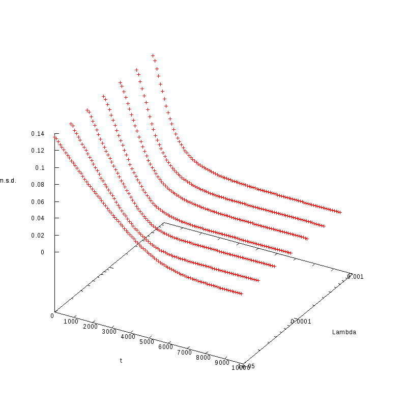
36%. The results are summarized in the following table. Again the results are plotted both
in 2D and 3D graphs.
The measurements have been taken for L = 100, 110, 120 and densities ranging from 1% to
36%. The results are summarized in the following table. Again the results are plotted both
in 2D and 3D graphs.
L=100
N=100
|

L=100
N=100
|
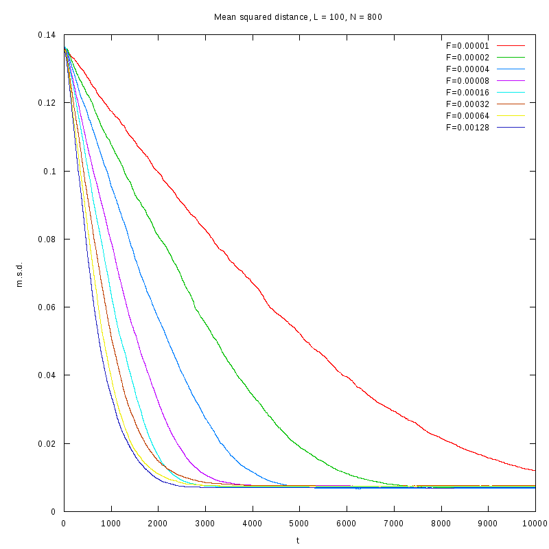
L=100
N=800
|

L=100
N=800
|
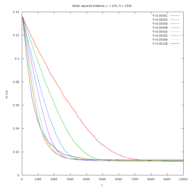
L=100
N=1500
|
L=100
N=1500
|
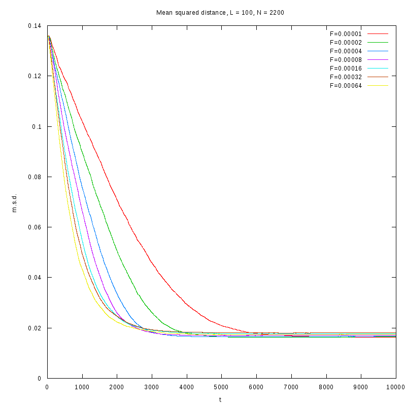
L=100
N=2200
|
L=100
N=2200
|
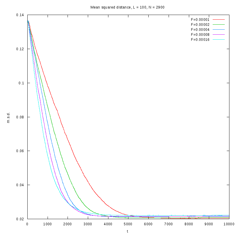
L=100
N=2900
|
L=100
N=2900
|
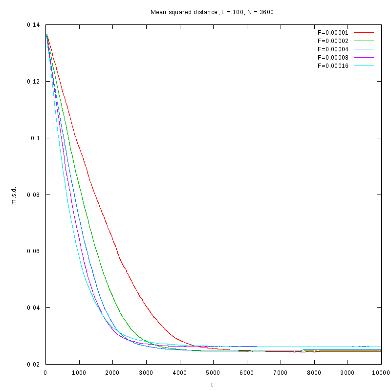
L=100
N=3600
|
L=100
N=3600
|
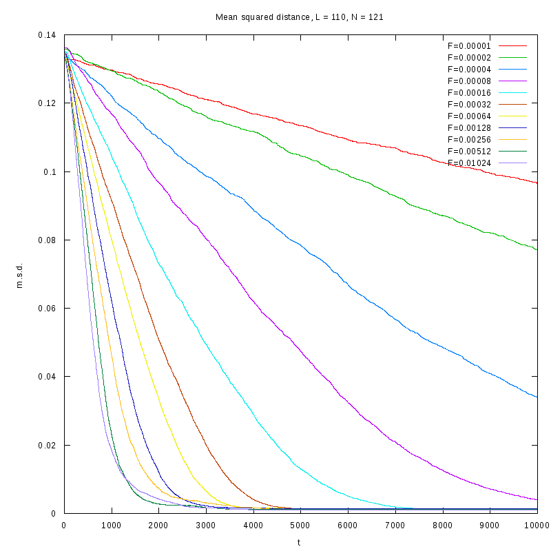
L=110
N=121
|
L=110
N=121
|
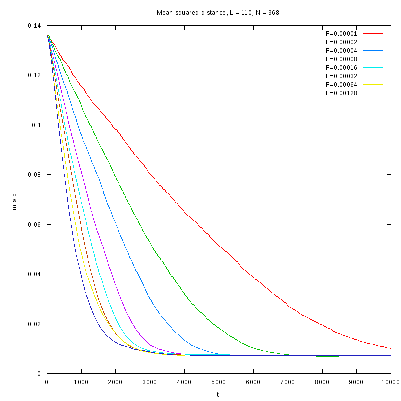
L=110
N=968
|

L=110
N=968
|
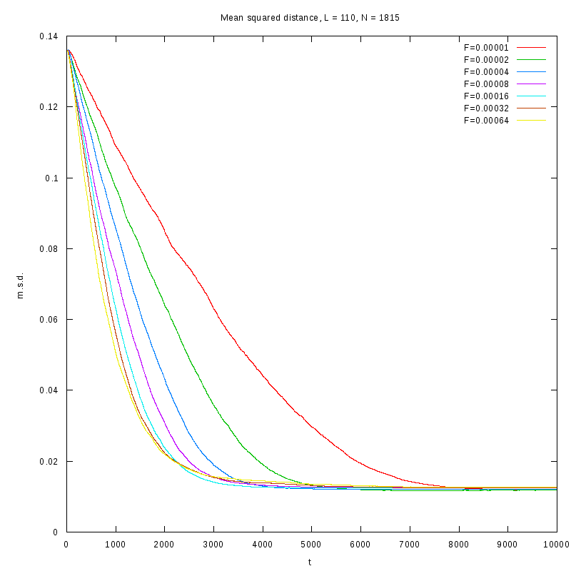
L=110
N=1815
|
L=110
N=1815
|
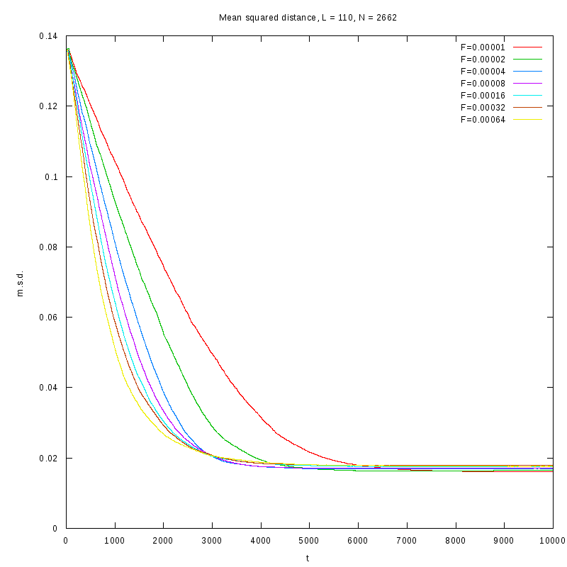
L=110
N=2662
|
L=110
N=2662
|
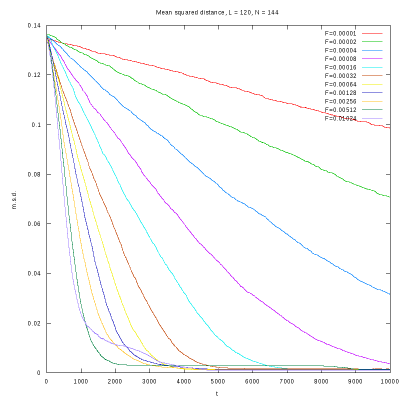
L=120
N=144
|

L=120
N=144
|
L=120
N=1152
|
L=120
N=1152
|
L=120
N=2160
|
L=120
N=2160
|
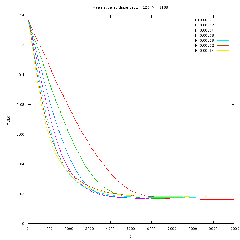
L=120
N=3168
|
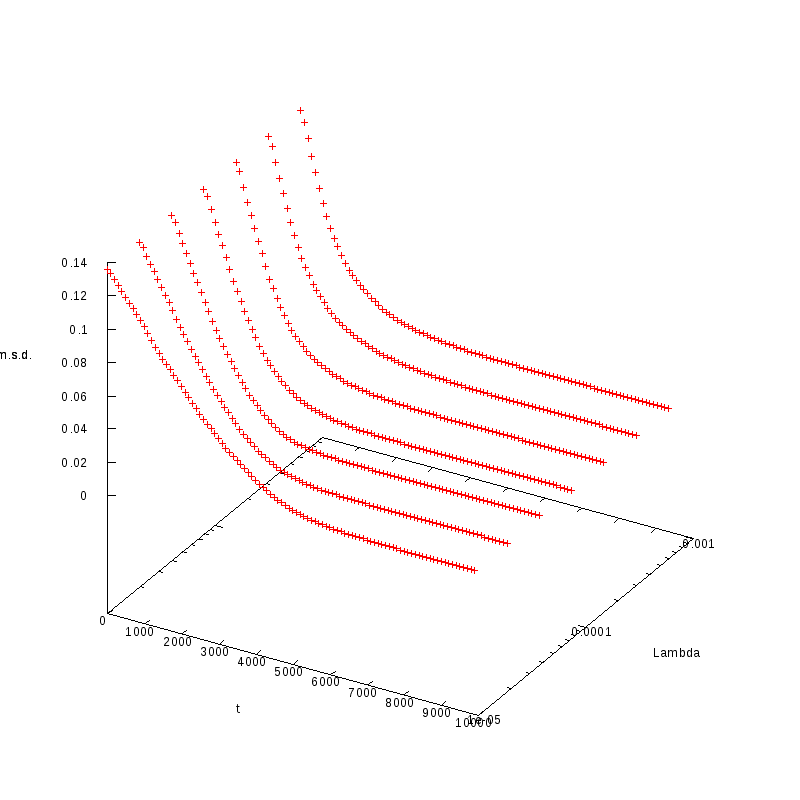
L=120
N=3168
|
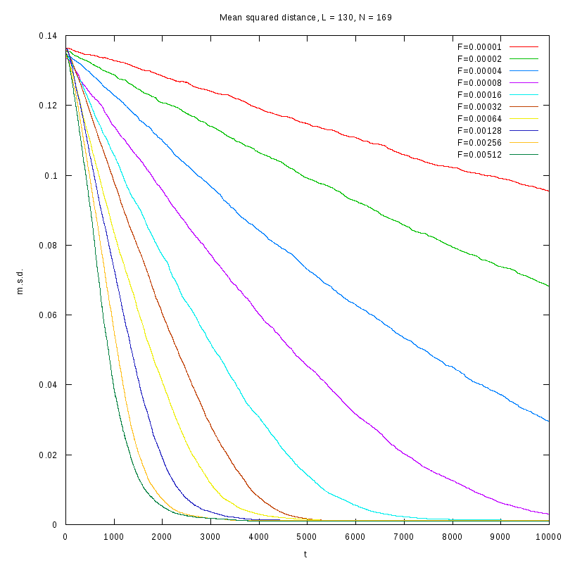
L=130
N=169
|
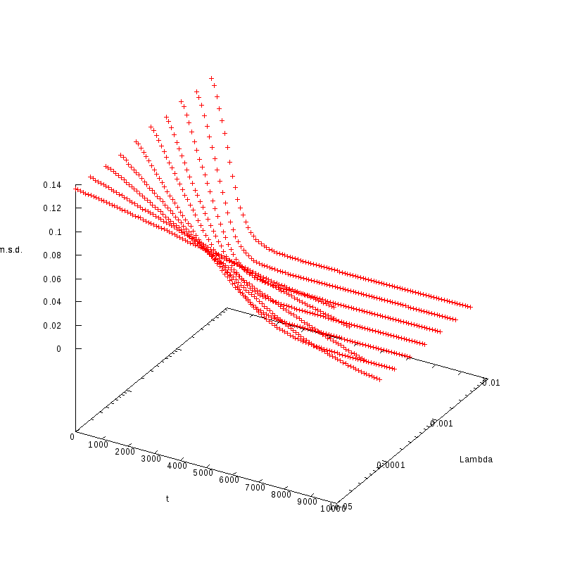
L=130
N=169
|
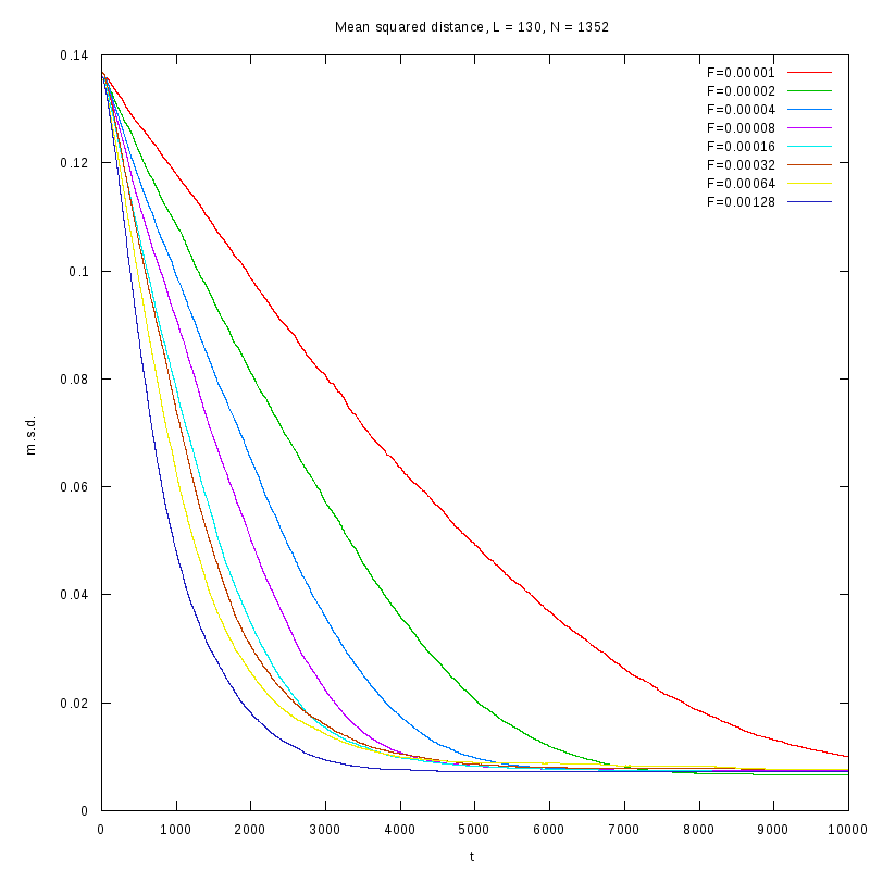
L=130
N=1352
|

L=130
N=1352
|
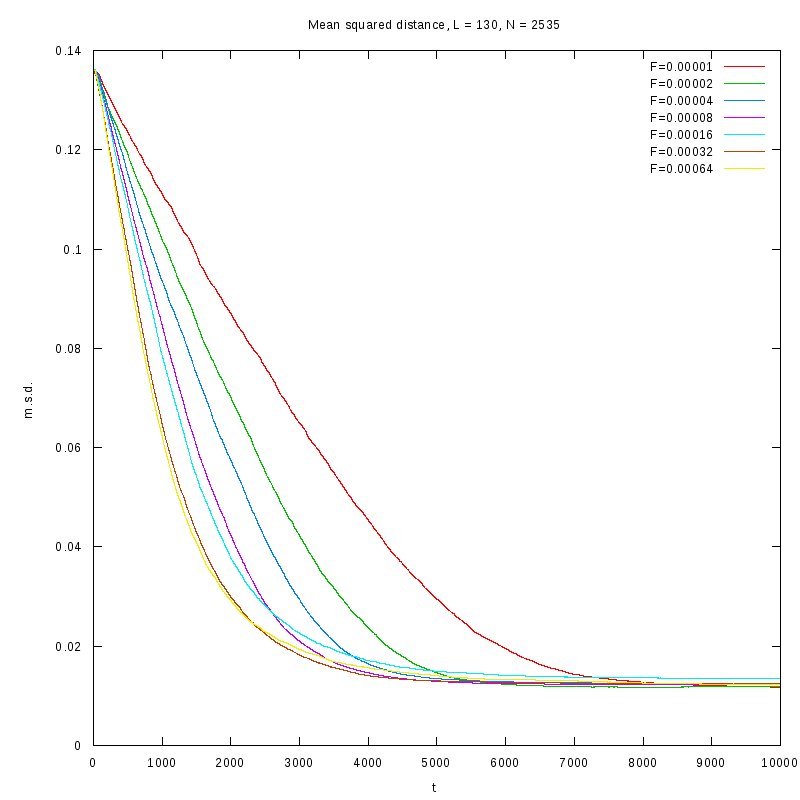
L=130
N=2535
|
L=130
N=2535
|
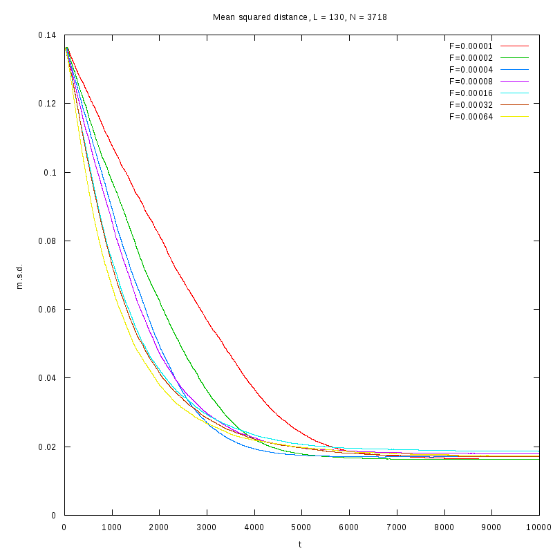
L=130
N=3718
|

L=130
N=3718
|
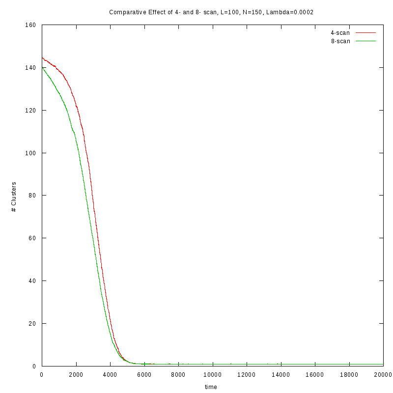
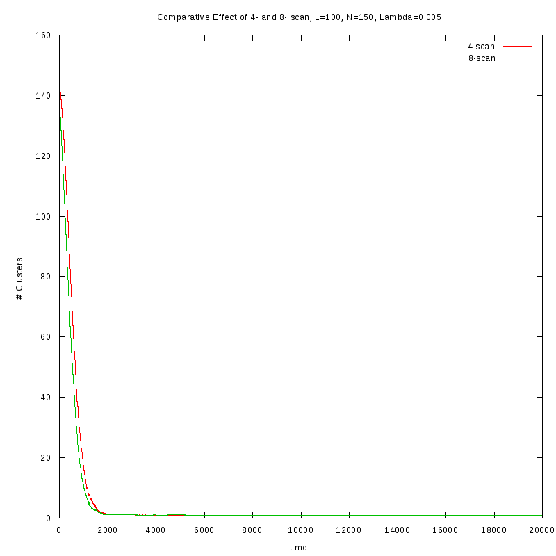
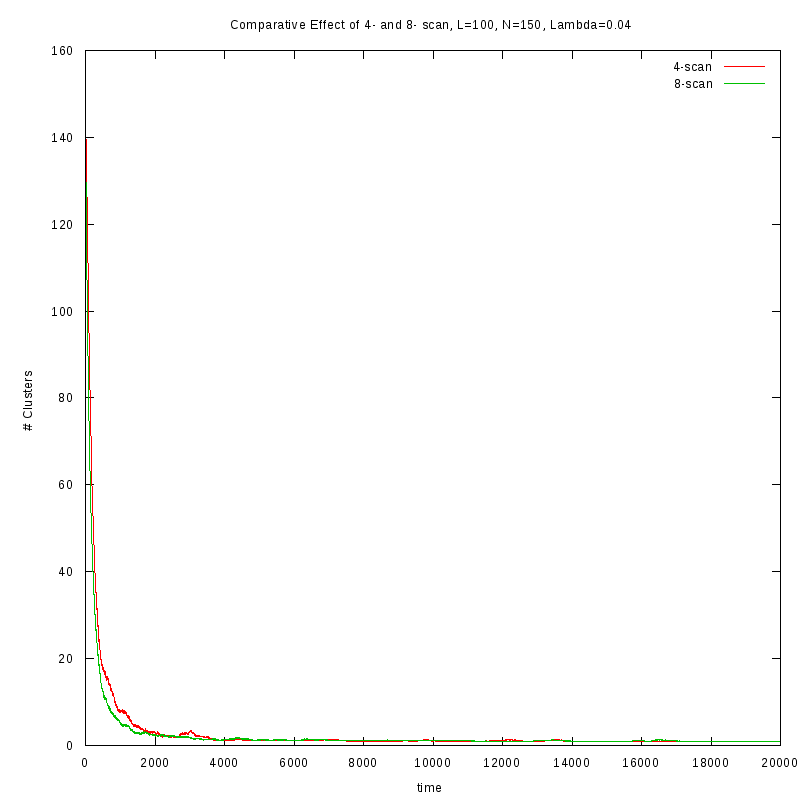
First results on the evolution of the number of clusters versus time
In this section we present some prelliminary results on the number of counted clusters
versus time for different values of
. In all cases N=150 and L=100.
We used two different cluster counting algorithms, one that is based on an 8-connected
neighborhood (i.e. two cells are taken to belong on the same cluster if they are in each
other's 8 connected neighborhood) and a 4-connected neighborhood.
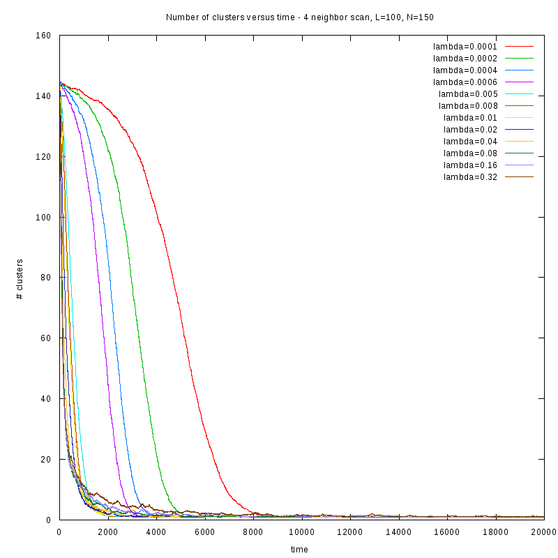
4-connected
|
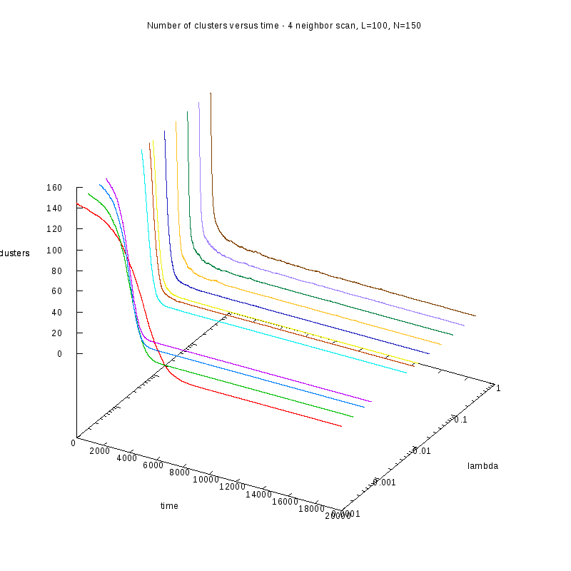
4-connected (3D)
|
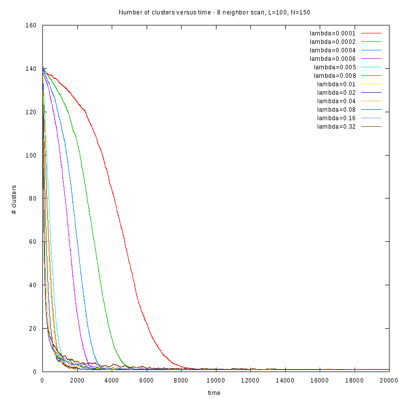
8-connected
|
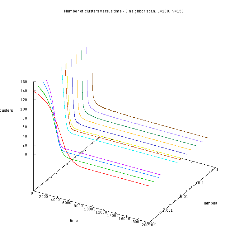
8-connected (3D)
|
One thing we should note here is that as
increases, we observe larger variations on the number
of clusters. This is caused by the formation of small clusters that persist through time.
When these small clusters “break” appart, the number of observed clusters increases
in order to stabilize again, as soon as they are absorbed by nearby clusters.
These variations are easier to observe on a logarithmic scale.
Comparison between the two cluster scan neighborhoods for different values of
As we observe from the above figures the 4-scan approach just differs from
the 8-scan by a (not necesarily constant) offset.
|